第 13 章 對數似然比 Log-likelihood ratio
對數似然比的想法來自於將對數似然方程圖形的 \(y\) 軸重新調節 (rescale) 使之最大值爲零。這可以通過計算該分佈方程的對數似然比 (log-likelihood ratio) 來獲得:
\[llr(\theta)=\ell(\theta|data)-\ell(\hat{\theta}|data)\]
由於 \(\ell(\theta)\) 的最大值在 \(\hat{\theta}\) 時, 所以,\(llr(\theta)\) 就是個當 \(\theta=\hat{\theta}\) 時取最大值,且最大值爲零的方程。很容易理解我們叫這個方程爲對數似然比,因爲這個方程就是將似然比 \(LR(\theta)=\frac{L(\theta)}{L(\hat{\theta})}\) 取對數而已。
之前我們也確證了,不包含我們感興趣的參數的方程部分可以忽略掉。還是用上一節 10人中4人患病的例子:
\[ L(\pi|X=4)=\binom{10}{4}\pi^4(1-\pi)^{10-4}\\ \Rightarrow \ell(\pi)=\log[\pi^4(1-\pi)^{10-4}]\\ \Rightarrow llr(\pi)=\ell(\pi)-\ell(\hat{\pi})=\log\frac{\pi^4(1-\pi)^{10-4}}{0.4^4(1-0.4)^{10-4}} \]
其實由上也可以看出 \(llr(\theta)\) 只是將對應的似然方程的 \(y\) 軸重新調節了一下而已。形狀是沒有改變的:
par(mfrow=c(1,2))
x <- seq(0,1,by=0.001)
y <- (x^4)*((1-x)^6)/(0.4^4*0.6^6)
z <- log((x^4)*((1-x)^6))-log(0.4^4*0.6^6)
plot(x, y, type = "l", ylim = c(0,1.1),yaxt="n",
     frame.plot = FALSE, ylab = "LR(\U03C0)", xlab = "\U03C0")
axis(2, at=seq(0,1, 0.2), las=2)
title(main = "Binomial likelihood ratio")
abline(h=1.0, lty=2)
segments(x0=0.4, y0=0, x1=0.4, y1=1, lty = 2)
plot(x, z, type = "l", ylim = c(-10, 1), yaxt="n", frame.plot = FALSE,
     ylab = "llr(\U03C0)", xlab = "\U03C0" )
axis(2, at=seq(-10, 0, 2), las=2)
title(main = "Binomial log-likelihood ratio")
abline(h=0, lty=2)
segments(x0=0.4, y0=-10, x1=0.4, y1=0, lty = 2)
圖 13.1: Binomial likelihood ratio and log-likelihood ratio
13.1 正態分佈數據的極大似然和對數似然比
假設單個樣本 \(y\) 是來自一組服從正態分佈數據的觀察值:\(Y\sim N(\mu, \tau^2)\)
那麼有:
\[ \begin{aligned} f(y|\mu) &= \frac{1}{\sqrt{2\pi\tau^2}}e^{(-\frac{1}{2}(\frac{y-\mu}{\tau})^2)} \\ \Rightarrow L(\mu|y) &=\frac{1}{\sqrt{2\pi\tau^2}}e^{(-\frac{1}{2}(\frac{y-\mu}{\tau})^2)} \\ \Rightarrow \ell(\mu)&=\log(\frac{1}{\sqrt{2\pi\tau^2}})-\frac{1}{2}(\frac{y-\mu}{\tau})^2\\ \text{omitting }&\;\text{terms not in}\;\mu \\ &= -\frac{1}{2}(\frac{y-\mu}{\tau})^2 \\ \Rightarrow \ell^\prime(\mu) &= 2\cdot[-\frac{1}{2}(\frac{y-\mu}{\tau})\cdot\frac{-1}{\tau}] \\ &=\frac{y-\mu}{\tau^2} \\ let \; \ell^\prime(\mu) &= 0 \\ \Rightarrow \frac{y-\mu}{\tau^2} &= 0 \Rightarrow \hat{\mu} = y\\ \because \ell^{\prime\prime}(\mu) &= \frac{-1}{\tau^2} < 0 \\ \therefore \hat{\mu} &= y \Rightarrow \ell(\hat{\mu}=y)_{max}=0 \\ llr(\mu)&=\ell(\mu)-\ell(\hat{\mu})=\ell(\mu)\\ &=-\frac{1}{2}(\frac{y-\mu}{\tau})^2 \end{aligned} \]
13.2 \(n\) 個獨立正態分佈樣本的對數似然比
假設一組觀察值來自正態分佈 \(X_1,\cdots,X_n\stackrel{i.i.d}{\sim}N(\mu,\sigma^2)\),先假設 \(\sigma^2\) 已知。將觀察數據 \(x_1,\cdots, x_n\) 標記爲 \(\underline{x}\)。 那麼:
\[ \begin{aligned} L(\mu|\underline{x}) &=\prod_{i=1}^nf(x_i|\mu)\\ \Rightarrow \ell(\mu|\underline{x}) &=\sum_{i=1}^n\text{log}f(x_i|\mu)\\ &=\sum_{i=1}^n[-\frac{1}{2}(\frac{x_i-\mu}{\sigma})^2]\\ &=-\frac{1}{2\sigma^2}\sum_{i=1}^n(x_i-\mu)^2\\ &=-\frac{1}{2\sigma^2}[\sum_{i=1}^n(x_i-\bar{x})^2+\sum_{i=1}^n(\bar{x}-\mu)^2]\\ \text{omitting }&\;\text{terms not in}\;\mu \\ &=-\frac{1}{2\sigma^2}\sum_{i=1}^n(\bar{x}-\mu)^2\\ &=-\frac{n}{2\sigma^2}(\bar{x}-\mu)^2 \\ &=-\frac{1}{2}(\frac{\bar{x}-\mu}{\sigma/\sqrt{n}})^2\\ \because \ell(\hat{\mu}) &= 0 \\ \therefore llr(\mu) &= \ell(\mu)-\ell(\hat{\mu}) = \ell(\mu) \end{aligned} \]
13.3 \(n\) 個獨立正態分佈樣本的對數似然比的分佈
假設我們用 \(\mu_0\) 表示總體均數這一參數的值。要注意的是,每當樣本被重新取樣,似然,對數似然方程,對數似然比都隨着觀察值而變 (即有自己的分佈)。
考慮一個服從正態分佈的單樣本 \(Y\): \(Y\sim N(\mu_0,\tau^2)\)。那麼它的對數似然比:
\[llr(\mu_0|Y)=\ell(\mu_0)-\ell(\hat{\mu})=-\frac{1}{2}(\frac{Y-\mu_0}{\tau})^2\]
根據卡方分佈 (Section 11) 的定義:
\[\because \frac{Y-\mu_0}{\tau}\sim N(0,1)\\ \Rightarrow (\frac{Y-\mu_0}{\tau})^2 \sim \mathcal{X}_1^2\\ \therefore -2llr(\mu_0|Y) \sim \mathcal{X}_1^2\]
所以,如果有一組服從正態分佈的觀察值:\(X_1,\cdots,X_n\stackrel{i.i.d}{\sim}N(\mu_0,\sigma^2)\),且 \(\sigma^2\) 已知的話:
\[-2llr(\mu_0|\bar{X})\sim \mathcal{X}_1^2\]
根據中心極限定理 (Section 8),可以將上面的結論一般化:
Theorem 13.1 如果 \(X_1,\cdots,X_n\stackrel{i.i.d}{\sim}f(x|\theta)\)。 那麼當重複多次從參數爲 \(\theta_0\) 的總體中取樣時,那麼統計量 \(-2llr(\theta_0)\) 會漸進於自由度爲 \(1\) 的卡方分佈: \[-2llr(\theta_0)=-2\{\ell(\theta_0)-\ell(\hat{\theta})\}\xrightarrow[n\rightarrow\infty]{}\;\sim \mathcal{X}_1^2\]
13.4 似然比信賴區間
如果樣本量 \(n\) 足夠大 (通常應該大於 \(30\)),根據上面的定理:
\[-2llr(\theta_0)=-2\{\ell(\theta_0)-\ell(\hat{\theta})\}\sim \mathcal{X}_1^2\]
所以:
\[Prob(-2llr(\theta_0)\leqslant \mathcal{X}_{1,0.95}^2=3.84) = 0.95\\ \Rightarrow Prob(llr(\theta_0)\geqslant-3.84/2=-1.92) = 0.95\]
故似然比的 \(95\%\) 信賴區間就是能夠滿足 \(llr(\theta)=-1.92\) 的兩個 \(\theta\) 值。
13.4.1 以二項分佈數據爲例
繼續用本文開頭的例子:
\[llr(\pi)=\ell(\pi)-\ell(\hat{\pi})=\log\frac{\pi^4(1-\pi)^{10-4}}{0.4^4(1-0.4)^{10-4}}\]
如果令 \(llr(\pi)=-1.92\) 在代數上可能較難獲得答案。然而從圖形上,如果我們在 \(y=-1.92\) 畫一條橫線,和該似然比方程曲線相交的兩個點就是我們想要求的信賴區間的上限和下限:
x <- seq(0,1,by=0.001)
z <- log((x^4)*((1-x)^6))-log(0.4^4*0.6^6)
plot(x, z, type = "l", ylim = c(-10, 1), yaxt="n", frame.plot = FALSE,
     ylab = "llr(\U03C0)", xlab = "\U03C0" )
axis(2, at=seq(-10, 0, 2), las=2)
abline(h=0, lty=2)
abline(h=-1.92, lty=2)
segments(x0=0.15, y0=-12, x1=0.15, y1=-1.92, lty = 2)
segments(x0=0.7, y0=-12, x1=0.7, y1=-1.92, lty = 2)
axis(1, at=c(0.15,0.7))
text(0.9, -1, "-1.92")
arrows(0.8, -1.92, 0.8, 0, lty = 1, length = 0.08)
arrows( 0.8, 0, 0.8, -1.92, lty = 1, length = 0.08)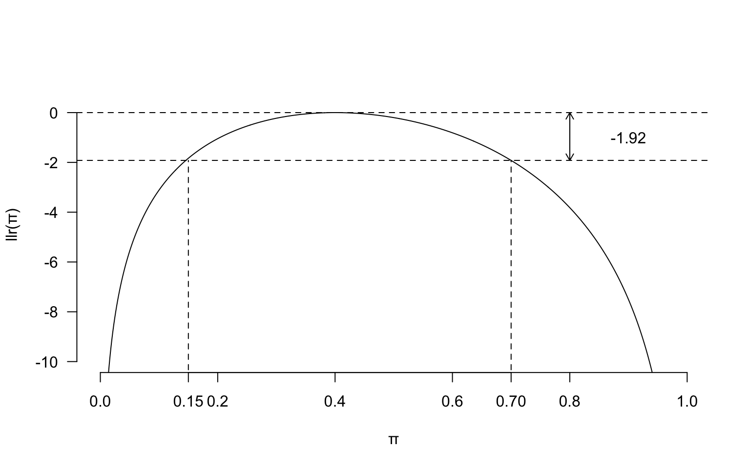
圖 13.2: Log-likelihood ratio for binomial example, with 95% confidence intervals shown
從上圖中可以讀出,\(95\%\) 對數似然比信賴區間就是 \((0.15, 0.7)\)
13.4.2 以正態分佈數據爲例
本文前半部分證明過, \(X_1,\cdots,X_n\stackrel{i.i.d}{\sim}N(\mu,\sigma^2)\),先假設 \(\sigma^2\) 已知。將觀察數據 \(x_1,\cdots, x_n\) 標記爲 \(\underline{x}\)。 那麼:
\[llr(\mu|\underline{x}) = \ell(\mu|\underline{x})-\ell(\hat{\mu}) = \ell(\mu|\underline{x}) \\ =-\frac{1}{2}(\frac{\bar{x}-\mu}{\sigma/\sqrt{n}})^2\]
很顯然,這是一個關於 \(\mu\) 的二次方程,且最大值在 MLE \(\hat{\mu}=\bar{x}\) 時取值 \(0\)。所以可以通過對數似然比法求出均值的 \(95\%\) 信賴區間公式:
\[-2\times[-\frac{1}{2}(\frac{\bar{x}-\mu}{\sigma/\sqrt{n}})^2]=3.84\\ \Rightarrow L=\bar{x}-\sqrt{3.84}\frac{\sigma}{\sqrt{n}} \\ U=\bar{x}+\sqrt{3.84}\frac{\sigma}{\sqrt{n}} \\ \text{note}: \;\sqrt{3.84}=1.96\]
注意到這和我們之前求的正態分佈均值的信賴區間公式 (Section 10.1) 完全一致。
13.5 Inference Practical 05
13.5.1 Q1
- 假設十個對象中有三人死亡,用二項分佈模型來模擬這個例子,求這個例子中參數 \(\pi\) 的似然方程和圖形 (likelihood) ?
解
\[\begin{aligned} L(\pi|3) &= \binom{10}{3}\pi^3(1-\pi)^{10-3} \\ \text{omitting } & \text{terms not in } \pi\\ \Rightarrow \ell(\pi|3) &= \log[\pi^3(1-\pi)^7] \\ &= 3\log\pi+7\log(1-\pi)\\ \Rightarrow \ell^\prime(\pi|3)&= \frac{3}{\pi}-\frac{7}{1-\pi} \\ \text{let} \; \ell^\prime& =0\\ &\frac{3}{\pi}-\frac{7}{1-\pi} = 0 \\ &\frac{3-10\pi}{\pi(1-\pi)} = 0 \\ \Rightarrow \text{MLE} &= \hat\pi = 0.3 \end{aligned}\]
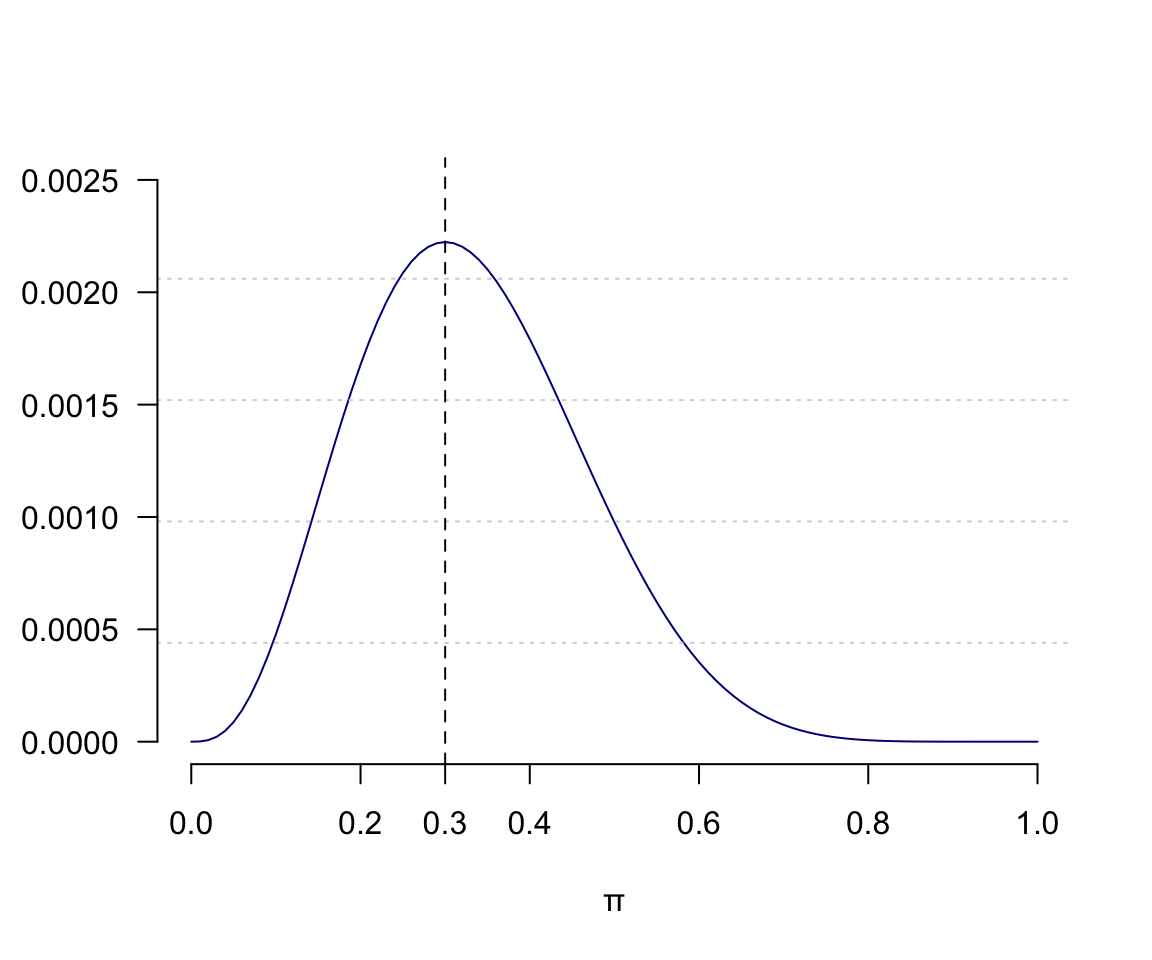
圖 13.3: Binomial likelihood function 3 out of 10 subjects
- 計算似然比,並作圖,注意方程圖形未變,\(y\) 軸的變化;取對數似然比,並作圖
## [1] 0.0000000 0.0004192 0.0031234 0.0098111 0.0216286 0.0392577plot(pi, LR, type = "l", ylim = c(0, 1),yaxt="n", col="darkblue",
frame.plot = FALSE, ylab = "", xlab = "\U03C0")
grid(NA, 5, lwd = 1)
axis(2, at=seq(0,1,0.2), las=2)
title(main = "Binomial likelihood ratio function\n 3 out of 10 subjects")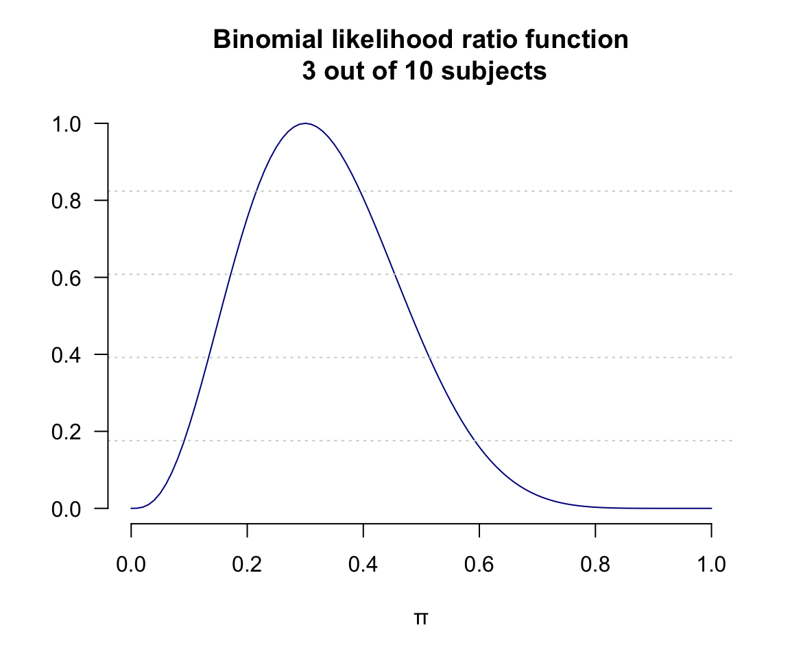
圖 13.4: Binomial likelihood ratio function 3 out of 10 subjects
logLR <- log(L/max(L))
plot(pi, logLR, type = "l", ylim = c(-4, 0),yaxt="n", col="darkblue",
     frame.plot = FALSE, ylab = "", xlab = "\U03C0")
grid(NA, 5, lwd = 1)
axis(2, at=seq(-4,0,1), las=2)
#title(main = "Binomial log-likelihood ratio function\n 3 out of 10 subjects")
abline(h=-1.92, lty=1, col="red")
axis(4, at=-1.92, las=0)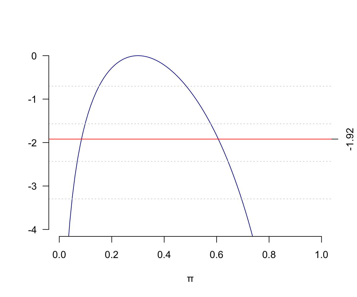
圖 13.5: Binomial log-likelihood ratio function 3 out of 10 subjects
13.5.2 Q2
- 與上面用同樣的模型,但是觀察人數變爲 \(100\) 人 患病人數爲 \(30\) 人,試作對數似然比方程之圖形,與上圖對比:
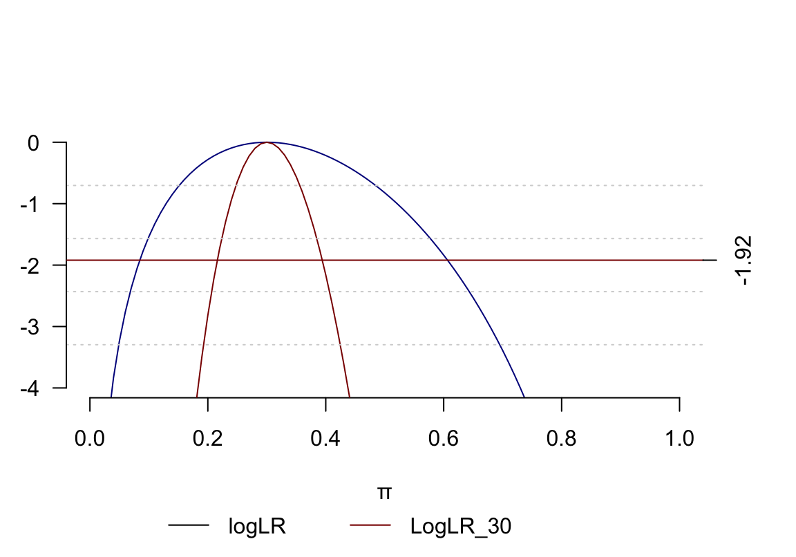
圖 13.6: Binomial log-likelihood ratio function 3 out of 10 and 30 out of 100 subjects
可以看出,兩組數據的 MLE 都是一致的, \(\hat\pi=0.3\),但是對數似然比方程圖形在 樣本量爲 \(n=100\) 時比 \(n=10\) 時窄很多,由此產生的似然比信賴區間也就窄很多(精確很多) 。所以對數似然比方程的曲率(二階導數) ,反映了觀察獲得數據提供的對總體參數 \(\pi\) 推斷過程中的信息量。而且當樣本量較大時,對數似然比方程也更加接近左右對稱的二次方程曲線。
13.5.3 Q3
在一個實施了160人年的追蹤調查中,觀察到8個死亡案例。使用泊松分佈模型,繪製對數似然比方程圖形,從圖形上目視推測極大似然比的 \(95\%\) 信賴區間。
解
\[\begin{aligned} d = 8, \;p &= 160\; \text{person}\cdot \text{year} \\ \Rightarrow \text{D}\sim \text{Poi}(\mu &=\lambda p) \\ L(\lambda|\text{data}) &= \text{Prob}(D=d=8) \\ &= e^{-\mu}\frac{\mu^d}{d!} \\ &= e^{-\lambda p}\frac{\lambda^d p^d}{d!} \\ \text{omitting}&\; \text{terms not in }\lambda \\ &= e^{-\lambda p}\lambda^d \\ \Rightarrow \ell(\lambda|\text{data})&= \log(e^{-\lambda p}\lambda^d) \\ &= d\cdot \log(\lambda)-\lambda p \\ & = 8\times \log(\lambda) - 160\times\lambda \end{aligned}\]
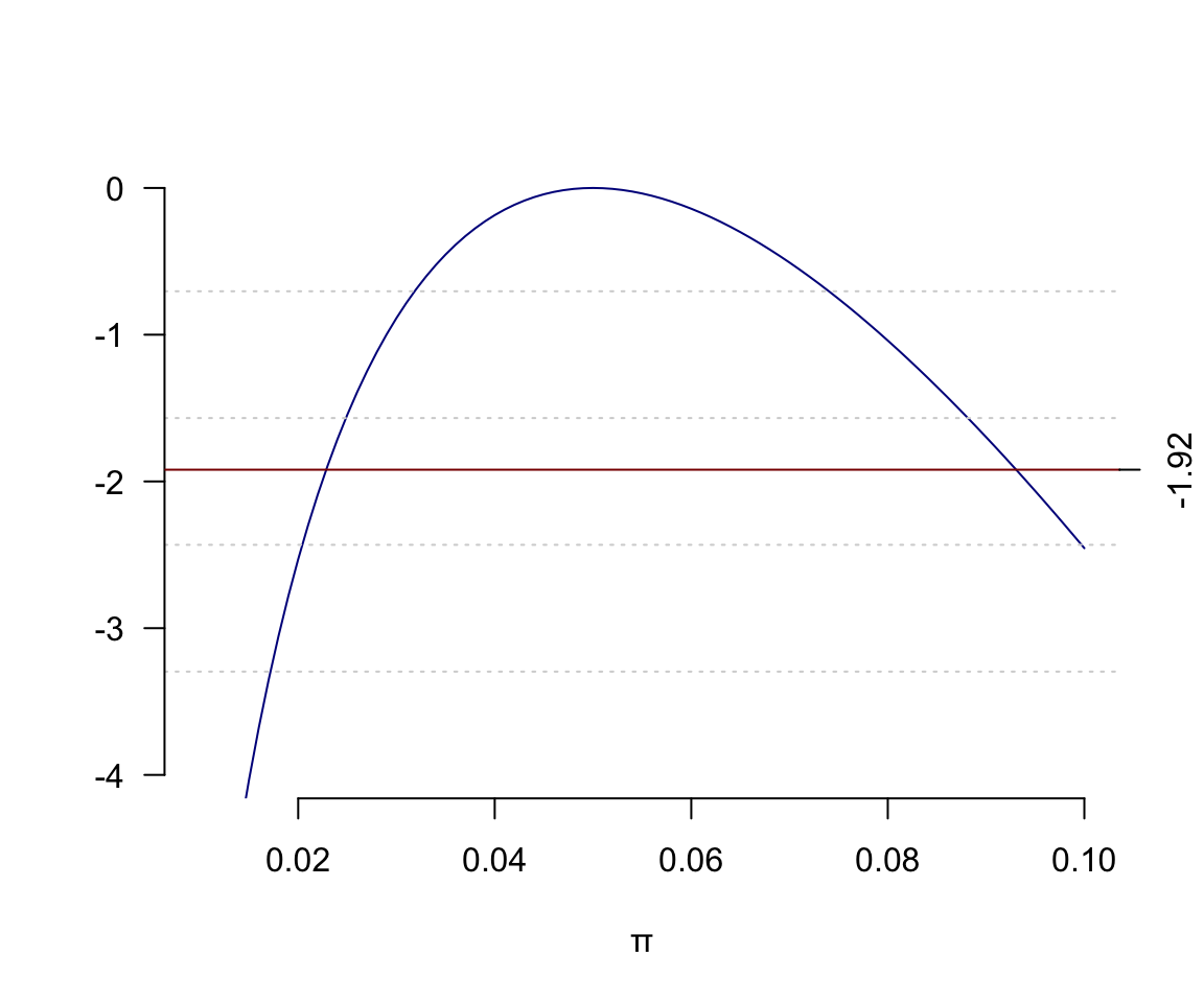
圖 13.7: Poisson log-likelihood ratio function 8 events in 160 person-years
| lambda | LogLR |
|---|---|
| 0.010 | -6.4755 |
| 0.011 | -5.8730 |
| 0.012 | -5.3369 |
| 0.013 | -4.8566 |
| 0.014 | -4.4237 |
| 0.015 | -4.0318 |
| 0.016 | -3.6755 |
| 0.017 | -3.3505 |
| 0.018 | -3.0532 |
| 0.019 | -2.7807 |
| 0.020 | -2.5303 |
| 0.021 | -2.3000 |
| 0.022 | -2.0878 |
| 0.023 | -1.8922 |
| 0.024 | -1.7118 |
| 0.025 | -1.5452 |
| 0.026 | -1.3914 |
| 0.027 | -1.2495 |
| 0.028 | -1.1185 |
| 0.029 | -0.9978 |
| 0.030 | -0.8866 |
| 0.031 | -0.7843 |
| 0.032 | -0.6903 |
| 0.033 | -0.6041 |
| 0.034 | -0.5253 |
| 0.035 | -0.4534 |
| 0.036 | -0.3880 |
| 0.037 | -0.3288 |
| 0.038 | -0.2755 |
| 0.039 | -0.2277 |
| 0.040 | -0.1851 |
| 0.041 | -0.1476 |
| 0.042 | -0.1148 |
| 0.043 | -0.0866 |
| 0.044 | -0.0627 |
| 0.045 | -0.0429 |
| 0.046 | -0.0271 |
| 0.047 | -0.0150 |
| 0.048 | -0.0066 |
| 0.049 | -0.0016 |
| 0.050 | 0.0000 |
| 0.051 | -0.0016 |
| 0.052 | -0.0062 |
| 0.053 | -0.0138 |
| 0.054 | -0.0243 |
| 0.055 | -0.0375 |
| 0.056 | -0.0534 |
| 0.057 | -0.0718 |
| 0.058 | -0.0926 |
| 0.059 | -0.1159 |
| 0.060 | -0.1414 |
| 0.061 | -0.1692 |
| 0.062 | -0.1991 |
| 0.063 | -0.2311 |
| 0.064 | -0.2651 |
| 0.065 | -0.3011 |
| 0.066 | -0.3389 |
| 0.067 | -0.3786 |
| 0.068 | -0.4201 |
| 0.069 | -0.4633 |
| 0.070 | -0.5082 |
| 0.071 | -0.5547 |
| 0.072 | -0.6029 |
| 0.073 | -0.6525 |
| 0.074 | -0.7037 |
| 0.075 | -0.7563 |
| 0.076 | -0.8103 |
| 0.077 | -0.8657 |
| 0.078 | -0.9225 |
| 0.079 | -0.9806 |
| 0.080 | -1.0400 |
| 0.081 | -1.1006 |
| 0.082 | -1.1624 |
| 0.083 | -1.2255 |
| 0.084 | -1.2896 |
| 0.085 | -1.3550 |
| 0.086 | -1.4214 |
| 0.087 | -1.4889 |
| 0.088 | -1.5575 |
| 0.089 | -1.6271 |
| 0.090 | -1.6977 |
| 0.091 | -1.7693 |
| 0.092 | -1.8419 |
| 0.093 | -1.9154 |
| 0.094 | -1.9898 |
| 0.095 | -2.0652 |
| 0.096 | -2.1414 |
| 0.097 | -2.2185 |
| 0.098 | -2.2964 |
| 0.099 | -2.3752 |
| 0.100 | -2.4548 |
所以從列表數據結合圖形, 可以找到信賴區間的下限在 0.022~0.023 之間, 上限在 0.093~0.094 之間。