第 102 章 貝葉斯等級回歸模型
102.1 關於等級迴歸模型
等級迴歸模型,指的是是一大類模型的設定,它也有很多不同的名字,例如多層模型(multilevel models),隨機效應模型(random effect models),隨機係數模型(random coefficient models),方差成分模型(variance-component models),混合效應模型(mixed effect models)。等級迴歸模型的最主要特點在於,這一類模型爲我們提供了一種正式的統計學框架,允許我們對複雜結構的數據進行恰當的統計分析,做出合理推斷。
等級迴歸模型最常見的情形可以是:
- 社會屬性上的:屬於相同家庭環境下的個人,成長於相似年代背景的一代人等各種社會網絡屬性;
- 地理屬性上的:在同一社區生活的人,同一城市,甚至是同一個國家生活的個體;
- 組織結構上的:如在同一個學校上學的學生,屬於同一個教育機構的工作人員等;
- 實驗設計上的:多中心,多地區合作的聯合臨牀實驗設計(mult-centre clinical trial);
- 時間序列上的:相同個體在不同時間點接受相同指標的測量獲得的一系列隨着時間變化而變化的數據。
另外,等級迴歸模型有幾個重要的概念需要澄清:
等級迴歸模型有助於考慮數據中的複雜結構 (modelling data with a complex structure)
數據的各種各樣的嵌套式結構可以通過等級迴歸模型體現出來,例如從屬於不同學校的學生,或者是在不同街道的家庭。等級迴歸模型有助於考慮數據的異質性 (heterogeneity)
等級迴歸模型不僅可以告訴我們常見的一般均值信息 (averages, i.e. provides the general relationships),等級迴歸模型還可以告訴我們不同等級之間的方差的異同 (variances),例如有些街道和另一些街道相比房價的差異變化更大,或者更小。等級迴歸模型又有助於考慮數據之間可能存在的非獨立性(依賴性,dependency)
許多數據它們本質上都不是相互獨立的,這種內在的依存性(也許是時間上,空間上,或者是周圍的環境相關的)可以通過等級迴歸模型來克服。例如,相同街區內的房屋價格,有理由認爲應該是有內在相關性的,它們更傾向於接近彼此的報價。等級迴歸模型可以幫助我們更加深刻的理解數據的內在的,微觀上的(micro)關係和外在結構上的,或者說宏觀 (macro) 層面上的關係。
例如,每個房屋的價格它的決定因素既有內在的影響因子,如房屋本身的性質,特徵,年份,主人等等;另外,決定它價格的可能還有它所在的街區,街道,小區,甚至是城市的特徵決定了它的價格。
正因爲我們所認知的數據本身,幾乎都可以有其內在的結構屬性,因此我們有理由使用理論和分析方法上更家貼近這種多層結構的統計學模型來瞭解這個世界。例如從國家層面上來說,可能有些國家的平均脂肪消費水平很高,有研究者發現這些國家比起另外脂肪消費量較低的國家來說,女性的乳腺癌發病率較高。但是,另外有些研究者可能發現,在一個國家內部,從個體與個體之間的脂肪攝入量上來觀察的話,又無法認可脂肪攝入量和乳腺癌發病呈現任何有意義的關係。
許多標準的統計學模型,都需要默認數據與數據之間,觀察對象與觀察對象之間有獨立性 (independent observation)。然而現實之中這一點經常是無法做到的。許多實際數據中你會發現默認對象之間的獨立性本身,是不合理的。因爲觀察對象之間可能存在的內在相關性,決定了一些觀察對象可能比起另外一些觀察對象更加傾向於有同質性。
那麼多層迴歸模型就是這樣一類能夠幫助我們理解數據結構的模型。它的靈活性體現在,
- 多層迴歸模型提供我們把相關性或者異質性部分的數據結構用模塊化的方法 (modular) 放入統計學模型中;
- 多層迴歸模型也會允許我們把數據中的缺失值,甚至是測量誤差給考慮進來,提供更加強有力(但是複雜的)統計學模型。
102.2 多層數據在模型中可能要用到的前提條件
在多層模型擬合多層數據時,有一個基本的問題就是如何正確地理解模型中各種各樣的回歸系數(參數, parameters):例如 \(J\) 個單位(可能是:個人,個體,子集 subset,區域,時間點,實驗組,等)的回歸參數 \(\theta_1, \dots, \theta_J\)。對這些回歸系數的正確理解,是要建立在對我們研究的問題,研究的數據的結構的理解之上的。
舉幾個簡單的例子來說,\(\theta_j\) 有可能有這樣的意義:
- 不同類型的患者(可以是不同的年齡組,疾病的分級,或者治療條件等)的治療效果;
- 在meta分析中則可以體現不同研究的研究效應(study effect);
- 某疾病在不同地區,年齡組,時間段的相對危險度;
- 在某些生長曲線模型 (growth curves models) 中的個體效應 (subject effect)。
綜上所述,我們可以發現,雖然多層回歸模型可能可以克服個體之間存在依賴性的問題,但是模型中的參數符合的前提條件可以有三種類別之分:
- 參數是相同的 (identical parameters);
- 參數是獨立的 (independent parameters);
- 參數是可交換的 (exchangeable parameters)。
下圖 102.1 展示了個體從屬於家庭醫生,家庭醫生又接着從屬於 Primary Care Trusts (PCTs) 的數據結構示意圖。
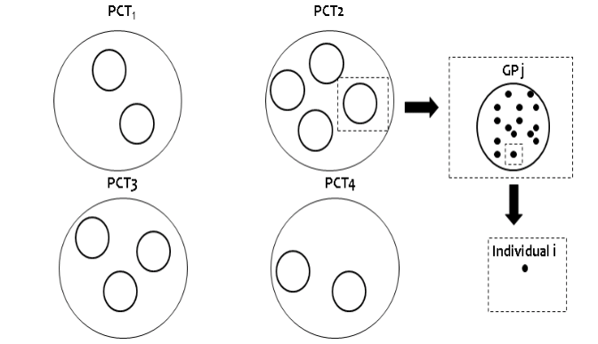
圖 102.1: GP example of multi-level structure: individuals within GPs within PCTs
102.2.1 參數是相同的 (identical parameters)
如果說參數相同的前提被認爲可以接受,那麼什麼 GP 什麼 PCT 的數據結構都可以被忽略,也就是每個個體都可以被視爲相互獨立的:
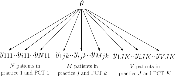
圖 102.2: GP example assuming identical parameters
但是,這意味着
- 一個參數可以產生全部的觀察對象 (one parameter generates all the observations);
- 參數\(\theta\)的估計會很容易,因爲全部觀察對象都被用來估計一個未知參數;
- 不能體現實際數據的層級結構情況 (it does not take into account differences in the PCT, GPs, etc.)
102.2.2 參數是獨立的 (independent parameters)
每一個參數如果要被認爲是全部沒有關聯(獨立)的話,如示意圖 102.3 所展現的那樣,每個GP都被單獨對待,即使同處在一個 PCT 的 GP 之間也被認爲是沒有任何相關聯信息的。
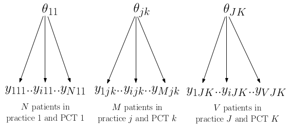
圖 102.3: GP example assuming independent parameters
102.2.3 參數是可交換的 (exchangeable parameters)
如果認爲參數是可置換的,那麼如圖 102.4 所示,這樣需要我們
- 對不同層級進行相應的分析;
- 認爲從屬於一個 PCT 的 GP 們更加彼此相似/接近,且他們的參數 \(\theta\) 通過共同的 \(\mu\) 來產生;
- 允許不同層級之間的參數信息可以相互交換,因爲他們通過數據結構互相鏈接。
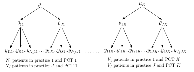
圖 102.4: GP example assuming exchangeable parameters
在較爲廣義的條件下(broad conditions),參數的可交換定義在數學上等價於認爲 \(\theta_1, \dots, \theta_J\) 來自於一個共同的先驗概率分佈 (common prior distribution),只是它的參數是未知的 (with unkown parameters)。
多層迴歸模型允許未知參數之間相互借鑑,取長補短 (borrowing of strength across units)。\(\theta_i\)的事後概率分佈事實上從全部的未知參數構成的似然中借取能量 (borrows stength from the likelihood function contributions for all the units, via their joint influence on the posterior estimates of the unknown hyper-parameters)。通過 MCMC 計算機模擬試驗的方法,加上多層迴歸模型對真實世界的模擬,統計估計的效率被大大提升了。別忘了, MCMC的靈活性同時讓我們可以放鬆對隨機效應要服從正態分佈這一前提條件。
可見,這第三種情形,參數的可交換性是進行多層模型分析的基石,而不是認爲未知參數是相互獨立或者完全相同。
構建多層迴歸模型本身提供了廣闊的視野,讓我們通過統計學工具一窺真實世界數據的複雜結構:
- 我們可以在模型中加入2層甚至更多層的數據結構;
- 允許加入非嵌套變量,交叉變量 (non-nested/cross-classified),例如不同GP的病人,他們參加治療的醫院或許各不相同。
- 同一對象的重複觀察值 (repeated observations),可以出現在一部分未知參數,或者全部未知參數中,然後我們通過線性或者非線性(廣義線性)隨機效應模型來表達其關係。
- 數據中的時間前後關係,甚至於是空間上的關係也可以通過多層迴歸模型來表達。
- 當然,你也可以在不同層級水平上增加需要考慮的共變量。
當我們在學習和建立複雜數據結構的模型時,貝葉斯統計學提供的強有力工具再一次印證了其高效且強大的分析效能。這裏我們僅有機會使用一個簡單的例子來展示如何在貝葉斯框架下構建擬合縱向研究數據的多層迴歸模型。
102.3 抗抑鬱臨牀試驗實例
102.3.1 縱向數據
縱向數據常見於對同一(單元的)樣本個體經過不同的時間點重複多次收集獲得的數據。一般來說,從同一個體收集的觀察數據相互之間存在依存關係。分析縱向數據可以有很多方法,但是不論哪種方法,都必須考慮到這個存在依存關係的數據結構。其中兩種最常見的手段分別是隨機效應線性迴歸模型 (random effects/hierarchical linear model) 和自迴歸模型 (autoregressive model)。這裏的實例我們使用隨機效應模型。
102.3.2 HAMD example
抗抑鬱臨牀試驗是一個有6個不同試驗中心,367名患者被隨機分配到3種治療方案。每名參加試驗的患者每週都會被使用 Hamilton depression score (HAMD) 評估打分,持續5周時間。其中 HAMD 分數範圍是 0-50 之間,分數越高,抑鬱症狀越嚴重。5周連續的HAMD打分過程是這樣的,第一次評分 (Week 0) 是在治療前,之後的4次打分是在治療開始之後 (Week 1-4)。這個數據之前曾經發表於文獻 (Diggle and Kenward 1994) 中。
實際上該試驗中從第二週開始就有患者退出治療 (dropout)。我們在這裏暫且忽略掉有患者中途退出這件事,先分析246名從頭至尾都完成了試驗的患者的數據。圖 102.5 展示的是完成全部試驗評分的患者中隨機選取50人的5次評分結果,按照時間的先後順序繪製的不同治療方案下每個人的分數變化軌跡,和每組治療方案的患者平均治療成績的軌跡。
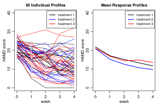
圖 102.5: HAMD data for complete cases
這個實驗中,我們關心的問題是三種治療方案對抑鬱症患者 HAMD 分數的變化的影響是否存在不同?
此時數據中的變量有:
- \(y\) HAMD 分數
- \(t\) 治療組
- \(w\) 治療周
這裏我們先暫且忽略掉試驗中心可能造成的不同療效,且假設HAMD評分隨着時間呈線性變化。那麼我們來思考或許可行的三個模型:
- 標準的簡單線性迴歸,非多層迴歸模型 (standard linear regression);
- 多層線性迴歸模型,且允許有隨機截距 (hierarchical model with random intercepts);
- 多層線性迴歸模型,且允許同時有隨機截距和隨機斜率兩種模型 (hierarchical mdoel with random intercepts and random slopes)。
102.3.3 貝葉斯簡單線性迴歸模型
爲此 HAMD 數據設定簡單線性迴歸模型如下:
- 患者的評分服從的概率分佈: \(y_{iw} \sim \text{Normal}(\mu_{iw}, \sigma^2)\),其中,\(y_{iw}\) 是第 \(i\) 名患者 在第 \(w, w \in \{0, 1, 2, 3, 4\}\) 周時的 HAMD 評分。
- 線性預測變量: \(\mu_{iw} = \alpha + \beta_{\text{treat}(i)}w\),其中,\(\text{treat}(i)\) 是第 \(i\) 名患者的治療組編號,可以取值 \(1,2,3\),\(w\) 則是周數,治療前爲第 \(w = 0\) 周,治療開始之後取 \(w = 1,2,3,4\) 周。
在簡單線性迴歸模型中,重複測量數據嵌套於 (nested) 每個患者個體這一事實被忽略了,我們爲每個未知參數加以無信息的先驗概率分佈:
\[ \begin{aligned} \alpha, \beta_1, \beta_2, \beta_2 & \sim \text{Normal}(0, 10000) \\ \frac{1}{\sigma^2} & \sim \text{Gamma}(0.001, 0.001) \end{aligned} \]
這個簡單線性迴歸模型對應的 BUGS 模型可以寫作:
for (i in 1:N){ # N individuals
    for (w in 1:W) { # W weeks
        hamd[i, w] ~ dnorm(mu[i, w], tau)
        mu[i, w] <- alpha + beta[treat[i]]*(w-1)
    }
# specification of priors
  alpha ~ dnorm(0, 0.00001)
  for (i in 1:T){ # T treatments
    beta[t]~dnorm(0, 0.00001)
  }
  tau ~ dgamma(0.001, 0.001)
  sigma.sq<-1/tau # normal errors
}
102.3.4 貝葉斯等級線性回歸–隨機截距模型
對簡單線性回歸模型進行適當修改之後就能直接把它引申爲隨機截距模型。其中,每一名患者都有自己的截距:
\[ \begin{aligned} y_{iw} & \sim \text{Normal}(\mu_{iw}, \sigma^2) \\ \mu_{iw} & = \alpha_i + \beta_{treat(i)}w \end{aligned} \]
此時模型中的前提是,以每名患者自己的截距 \(\alpha_i\) 爲條件時 (conditional on),患者的HAMD測試結果 \(\{y_{iw}, w = 0, \dots, 4\}\) 會相互獨立。同時,我們還假設所有的隨機截距 \(\alpha_i\) 服從相同的(共同的)先驗概率分佈。
\[ \alpha_i \sim \text{Normal}(\mu_\alpha, \sigma^2_\alpha) \;\; i = 1, \dots, 246 \]
這裏我們又假定了每個人的均值(截距)是來自相同分佈(可以互換的,exchangeability)。
再接下來,對於人羣的截距這一數據設定非常模糊的先驗概率超參數 (hyperparameters):
\[ \begin{aligned} \mu_\alpha & \sim \text{Normal}(0, 10000) \\ \sigma_\alpha & \sim \text{Uniform}(0, 100) \end{aligned} \]
這是一個典型的多層線性回歸模型 (Hierarchical LM or Linear Mixed Model, LMM),或者又叫做隨機截距模型(Random Intercepts model)。
這個模型可以使用BUGS語言描述如下:
for (i in 1:N) { # N individuals
    for (w in 1:W) { # W weeks
        hamd[i, w] ~ dnorm(mu[i,w], tau)
        mu[i,w] <- alpha[i] + beta[treat[i]]*(w-1)
    }
    alpha[i] ~ dnorm(alpha.mu, alpha.tau) # random intercepts
}
   # Specification of priors
alpha ~ dnorm(0, 0.00001)
alpha.mu ~ dnorm(0, 0.00001)
alpha.sigma ~ dunif(0, 100)
alpha.sigma.sq <- pow(alpha.sigma, 2)
alpha.tau <- 1/alpha.sigma.sq

for (t in 1:T){ # T treatments
    beta[t] ~ dnorm(0, 0.00001)
}
tau ~ dgamma(0.001, 0.001)
sigma.sq <- 1/tau  # Normal errors
無隨機截距的簡單線性回歸模型,和包括了隨機截距模型的多層線性回歸模型之間的差別,用 DAG 圖來表示可以直觀的展示如下:
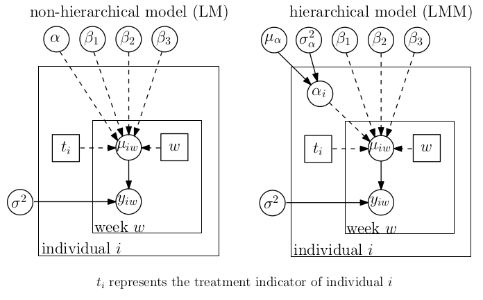
圖 102.6: DAGs for models for the HAMD example
102.3.5 貝葉斯等級線性回歸模型–隨機截距和隨機斜率模型
與隨機截距模型相類似地,我們可以把該模型從隨機截距的基礎上再擴展到隨機斜率模型,也就是可以認爲每名患者的HAMD分數變化的直線的斜率可以因人而異。
\[ \begin{aligned} y_{iw} & \sim \text{Normal}(\mu_{iw}, \sigma^2) \\ \mu_{iw} & = \alpha_i + \beta_{treat(i), i}w \end{aligned} \]
模型中的隨機截距\(\{\beta_{(1,i)}\}, \{\beta_{(2,i)}\}, \{\beta_{(3,i)}\}\), 同隨機截距 \(\{\alpha_i\}\) 一樣我們都賦予其相同的且模糊的無有效信息的先驗概率分佈:
這個隨機效應模型的BUGS模型代碼寫作如下:
for (i in 1:N) { # N individuals
    for (w in 1:W) { # W weeks
        hamd[i, w] ~ dnorm(mu[i, w], tau)
        mu[i, w] <- alpha[i] + beta[treat[i], i] * (w - 1)
    }
    alpha[i] ~ dnorm(alpha.mu, alpha.tau)
    for(t in 1:T) {beta[t, i] ~ dnorm(beta.mu[t], beta.tau[t])}
}

# Priors
for (t in 1:T) { # T treatments
    beta.mu[t] ~ dnorm(0, 0.0001)
    beta.sigma[t] ~ dunif(0, 100)
    beta.sigma.sq[t] <- pow(beta.sigma[t], 2)
    beta.tau[t] <- 1/beta.sigma.sq[t]
}

# specification of other priors as before in the random intercept model
alpha ~ dnorm(0, 0.00001)
alpha.mu ~ dnorm(0, 0.00001)
alpha.sigma ~ dunif(0, 100)
alpha.sigma.sq <- pow(alpha.sigma, 2)
alpha.tau <- 1/alpha.sigma.sq

for (t in 1:T){ # T treatments
    beta[t] ~ dnorm(0, 0.00001)
}
tau ~ dgamma(0.001, 0.001)
sigma.sq <- 1/tau  # Normal errors
102.3.6 HAMD 數據不同模型結果的比較
- 在非隨機效應模型(即簡單線性回歸模型)中,
- 一共有3條回歸直線被統計模型擬合,其中每個治療方案爲一條回歸直線;
- 每個治療方案獲得的回歸直線本身,具有相同的截距;
- 每個治療方案的回歸直線具有不同的斜率。
- 在隨機截距模型中,
- 每名參加實驗的患者有自己的回歸直線;
- 每名患者的回歸直線只有自己的隨機截距,也就是HAMD的起始值被允許取不同的值。
- 再隨機截距隨機斜率模型中,
- 每名患者的回歸直線被允許擁有不同的斜率,和不同的截距。
下圖(表) 102.7 提供了三種不同模型分析 HAMD 數 據結果的報告。可以注意到當模型中增加隨機效應時,明顯地,殘差方差 (residual variance) \(\sigma^2\) 大幅下降。因爲這些使用簡單線性回歸模型 時只能被歸類到一個隨機殘差當中去的方差,分別被歸類到了隨機截距的方差, 和隨機斜率的方差中去了。三個模型的 DIC 指標也提示我們,該數據更加支持 隨機效應模型,且兩個隨機效應模型相比,隨機截距和隨機斜率都有的隨機效應 模型更加貼合收集來的觀測數據。同時表格的最下面也列出了每個不同模型中實 際使用到的有效變量個數 (effective number of parameters, \(p_D\)),而且這 個有效變量個數隨着隨機效應的增加而顯著增加。
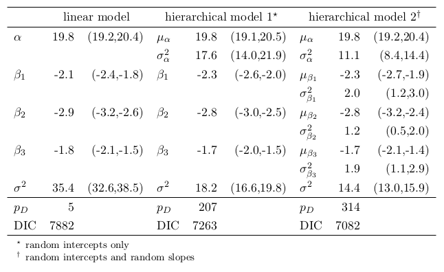
圖 102.7: Posterior mean (95% credible intervals) for the non-hierarchical and hierarchical models fitted to the HAMD data.
102.3.7 HAMD 數據實例結果的解釋
值得注意的是,在 HAMD 數據中,我們關心的實驗問題其實是,“三種不同治療方案,對於HAMD分析得分的變化(也就是回歸線的斜率),是否起到不同的作用。(whether there are any difference in the effects of the 3 treatments on the change in HAMD score over time)”。也就是說我們特別對斜率的不同感興趣。
- \(\beta_1 - \beta_2, \beta_1 - \beta_3, \beta_2 - \beta_3\);
- 以及隨機斜率模型中的:\(\mu_{\beta_1} - \mu_{\beta_2}, \mu_{\beta_1} - \mu_{\beta_3}, \mu_{\beta_2} - \mu_{\beta_3}\)
這些斜率差值其實可以通過 BUGS 代碼簡單方便的計算出來,便於我們進行樣本採集和統計推斷:
# calculate contrasts
contrasts[1] <- beta[1] - beta[2]
contrasts[2] <- beta[1] - beta[3]
contrasts[3] <- beta[2] - beta[3]
或者寫成:
contrasts[1] <- beta.mu[1] - beta.mu[2]
...三個不同模型的斜率比較結果總結如下圖(表)102.8,其中隨機即截距隨機斜率模型的三個斜率比較的事後概率分佈圖繪製如圖102.9。由於 HAMD 得分越低表示抑鬱症症狀越輕,所以表格中的斜率差如果是負的,表示斜率比較中前者的療效更好(下降效果更顯著),如果斜率差是正的,那麼就是反過來證明斜率比較中後者的療效更好。所以很顯然,療法2比起療法1對於 HAMD 分數的下降更加有顯著效果。這個結果和之前對數據的粗略均值繪製圖102.5提示的結果相一致。當然一個更加完整的貝葉斯統計學分析還要包括對模型進行擬合診斷,以及對模型進行更加仔細的推敲(例如對線性變量中心化,或者增加實驗設施這個層級的隨機效應,或者允許增加非線性的結果)。另外值得注意的是,我們之前介紹過的所有對於非多層回歸模型的擬合檢查在混合效應模型中都會變得更加複雜。還有值得提醒的一點在於,DIC在大部分模型擬合中都可以用於比較不同的模型,但是有時候也會出現 BUGS 軟件無法計算 DIC 的情況。先驗概率分佈的選擇也是混合效應模型擬合時需要慎重考慮的一點,這些內容這裏由於篇幅限制無法一一詳細介紹。
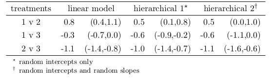
圖 102.8: Posterior mean (95% credible interval) for the contrasts (treatment comparisons) from models fitted to the HAMD data
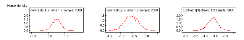
圖 102.9: Density plots for the hierarchical model with random intercepts and random slopes.
102.4 Practical Bayesian Statistics 08
本章練習題會延續使用前一個章節 (Chapter 101.5) 中使用的練習題數據,岡比亞兒童使用蚊帳睡眠是否能夠降低或者減輕瘧疾。
- 把前章練習中的貝葉斯邏輯回歸模型改造成爲一個包含村莊級別隨機效應的多層邏輯回歸模型。
# Logistic regression model for malaria data

model {
   for(i in 1:149) {
      MALARIA[i] ~ dbin(p[i], POP[i])
      logit(p[i]) <- alpha + beta.age[AGE[i]] +
                            beta.bednet[BEDNET[i]] +
                            beta.green*(GREEN[i] - mean(GREEN[])) +
                            beta.phc*PHC[i] +
                            theta[VILLAGE[i]]
   }
   # village-level random effect
   for (j in 1:25) {
       theta[j] ~ dnorm(0, tau)
       OR.village[j]  <- exp(theta[j])
       # Odds ratio of malaria in village j relative to the average
   }


   # vague priors on regression coefficients
   alpha ~ dnorm(0, 0.00001)
   sigma ~ dunif(0, 100)
   tau <- 1/pow(sigma, 2)
   beta.age[1] <- 0
       # set coefficient for baseline age group to zero (corner point constraint)
   beta.age[2] ~ dnorm(0, 0.00001)
   beta.age[3] ~ dnorm(0, 0.00001)
   beta.age[4] ~ dnorm(0, 0.00001)
   beta.bednet[1] <- 0
       # set coefficient for baseline bednet group to zero (corner point constraint)
   beta.bednet[2] ~ dnorm(0, 0.00001)
   beta.bednet[3] ~ dnorm(0, 0.00001)
   beta.green ~ dnorm(0, 0.00001)
   beta.phc ~ dnorm(0, 0.00001)

   # calculate odds ratios of interest
   OR.age[2] <- exp(beta.age[2]) # OR of malaria for age group 2 vs. age group 1
   OR.age[3] <- exp(beta.age[3]) # OR of malaria for age group 3 vs. age group 1
   OR.age[4] <- exp(beta.age[4]) # OR of malaria for age group 4 vs. age group 1

   OR.bednet[2] <- exp(beta.bednet[2]) # OR of malaria for children using untreated bednets vs. not using bednets
   OR.bednet[3] <- exp(beta.bednet[3]) # OR of malaria for children using treated bednets vs. not using bednets
   OR.bednet[4] <- exp(beta.bednet[3] - beta.bednet[2]) # OR of malaria for children using treated bednets vs. using untreated bednets
   OR.green <- exp(beta.green)  # OR of malaria per unit increase in greenness index of village
   OR.phc <- exp(beta.phc)      # OR of malaria sfor children living in villages belonging to the primary health care system versus children living in villages not in the health care system
   logit(baseline.prev) <- alpha # baseline prevalence of malaria in baseline group (i.e. child in age group 1, sleeps without bednet, and lives in a village with average greenness index and not in the health care system)

   PP.untreated <- step(1 - OR.bednet[2]) # probability that using untreated bed net vs. no bed net reduces odds of malaria
   PP.treated <- step(1- OR.bednet[4]) # probability that using treated vs. untreated bednet reduces odds of malaria
}
# Read in the data:
# Data <- read_delim(paste(bugpath, "/backupfiles/malaria-data.txt", sep = ""), delim = " ")
Data <- read.table(paste(bugpath, "/backupfiles/malaria-data.txt", sep = ""),
header = TRUE)
# Data file for the model
Dat <- list(
POP = Data$POP,
MALARIA = Data$MALARIA,
AGE = Data$AGE,
BEDNET = Data$BEDNET,
GREEN = Data$GREEN,
PHC = Data$PHC,
VILLAGE = Data$VILLAGE
)
# initial values for the model
# the choice is arbitrary
inits <- list(
list(alpha = -0.51,
beta.age = c(NA, 0.83, 0.28, -1.68),
beta.bednet = c(NA, -2.41, 0.68),
beta.green = -0.23,
beta.phc = 1.82,
sigma = 3),
initlist1 <- list(alpha = 1.29,
beta.age = c(NA, 0.49, -0.38, -0.04),
beta.bednet = c(NA, 6.85, 0.09),
beta.green = 2.66,
beta.phc = -0.31,
sigma = 1)
)
# Set monitors on nodes of interest
parameters <- c("OR.age", "OR.bednet", "OR.green", "OR.phc", "PP.treated", "PP.untreated", "baseline.prev", "sigma", "OR.village")
# fit the model in jags
jagsModel <- jags(data = Dat,
model.file = paste(bugpath,
"/backupfiles/malaria-model-hierarchical.txt",
sep = ""),
parameters.to.save = parameters,
n.iter = 1000,
n.chains = 2,
inits = inits,
n.burnin = 0,
n.thin = 1,
progress.bar = "none")## Compiling model graph
## Resolving undeclared variables
## Allocating nodes
## Graph information:
## Observed stochastic nodes: 149
## Unobserved stochastic nodes: 34
## Total graph size: 1435
##
## Initializing model# Show the trace plot
Simulated <- coda::as.mcmc(jagsModel)
ggSample <- ggs(Simulated)
ggSample %>%
filter(Parameter %in% c("OR.age[2]", "OR.age[3]", "OR.age[4]",
"OR.bednet[2]", "OR.bednet[3]", "OR.bednet[4]",
"OR.green", "baseline.prev", "OR.phc", "OR.village[1]")) %>%
ggs_traceplot()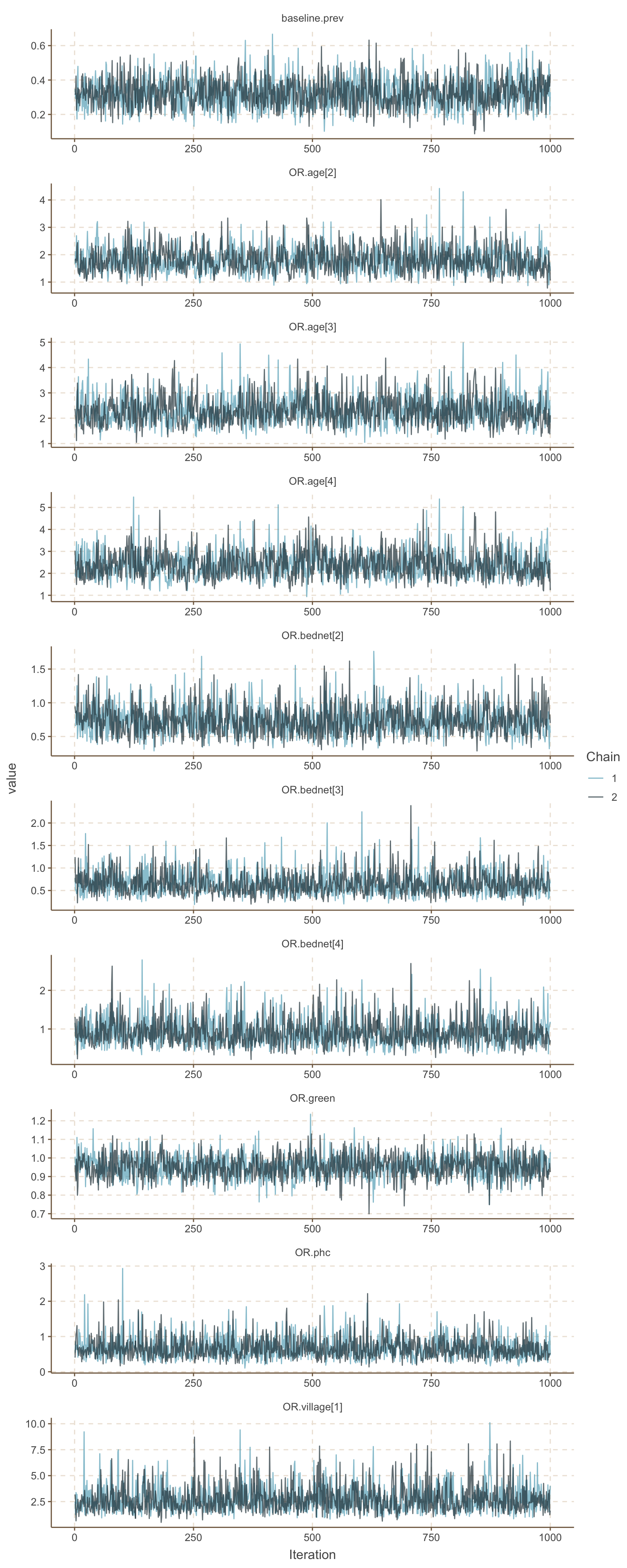
圖 102.10: Density plots for parameters for hierarchical GLM about the odds of malaria regarding netbeds use in Gambia children.
## Potential scale reduction factors:
##
##                Point est. Upper C.I.
## OR.age[2]           1.000      1.000
## OR.age[3]           0.999      0.999
## OR.age[4]           1.000      1.004
## OR.bednet[2]        1.002      1.005
## OR.bednet[3]        1.002      1.010
## OR.bednet[4]        1.001      1.008
## OR.green            1.001      1.003
## OR.phc              1.003      1.005
## OR.village[1]       0.999      1.000
## OR.village[2]       1.002      1.002
## OR.village[3]       1.000      1.004
## OR.village[4]       1.003      1.003
## OR.village[5]       1.002      1.004
## OR.village[6]       1.002      1.008
## OR.village[7]       0.999      0.999
## OR.village[8]       1.004      1.004
## OR.village[9]       1.023      1.039
## OR.village[10]      1.000      1.004
## OR.village[11]      1.003      1.018
## OR.village[12]      1.011      1.020
## OR.village[13]      1.003      1.005
## OR.village[14]      1.011      1.034
## OR.village[15]      1.002      1.007
## OR.village[16]      1.000      1.000
## OR.village[17]      1.012      1.045
## OR.village[18]      1.004      1.005
## OR.village[19]      1.030      1.038
## OR.village[20]      1.001      1.002
## OR.village[21]      1.000      1.003
## OR.village[22]      1.001      1.001
## OR.village[23]      1.002      1.006
## OR.village[24]      1.014      1.014
## OR.village[25]      1.016      1.018
## PP.treated          0.999      1.001
## PP.untreated        1.008      1.019
## baseline.prev       1.000      1.001
## deviance            1.000      1.001
## sigma               0.999      0.999
##
## Multivariate psrf
##
## 1.04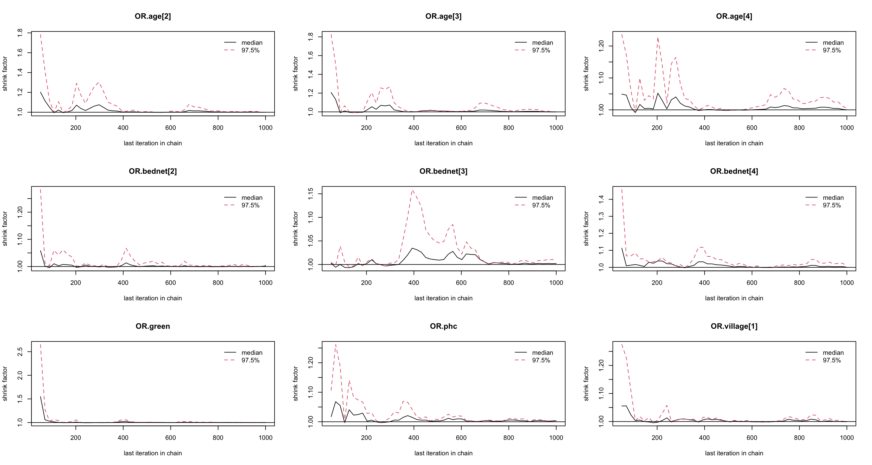
圖 102.11: Gelman-Rubin convergence statistic of parameters for GLM about the odds of malaria regarding netbeds use in Gambia children.
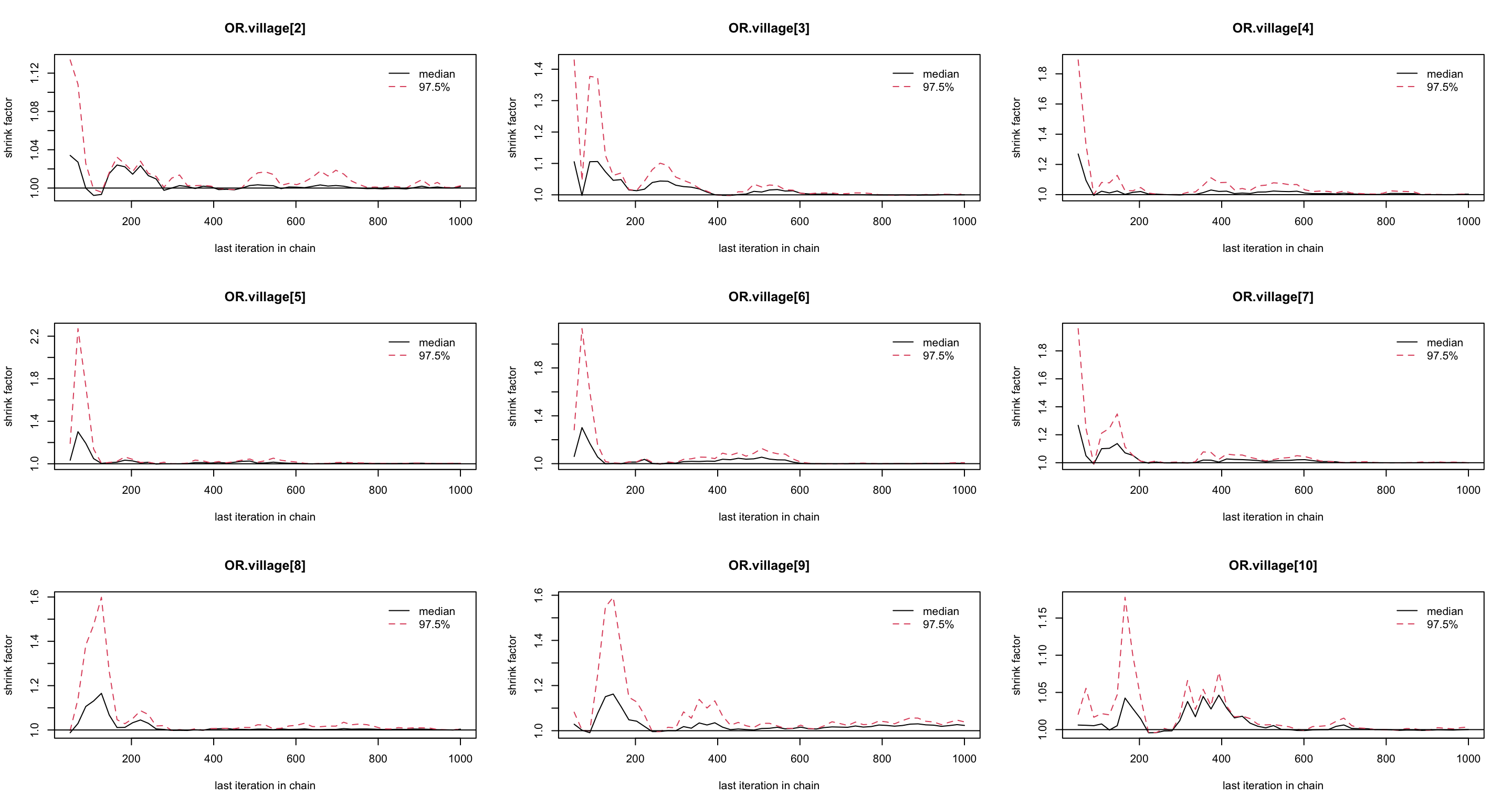
圖 102.12: Gelman-Rubin convergence statistic of parameters for GLM about the odds of malaria regarding netbeds use in Gambia children.
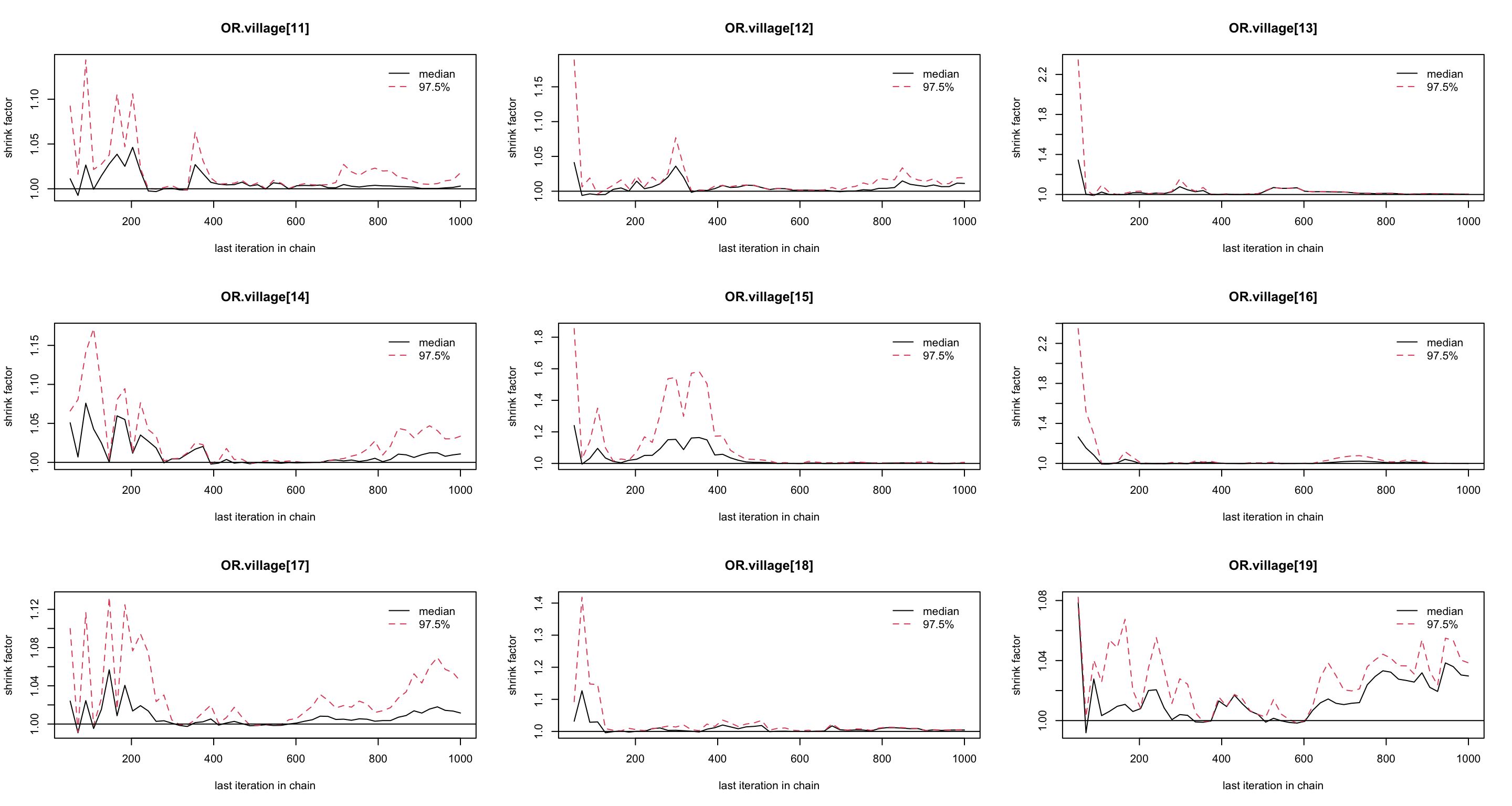
圖 102.13: Gelman-Rubin convergence statistic of parameters for GLM about the odds of malaria regarding netbeds use in Gambia children.
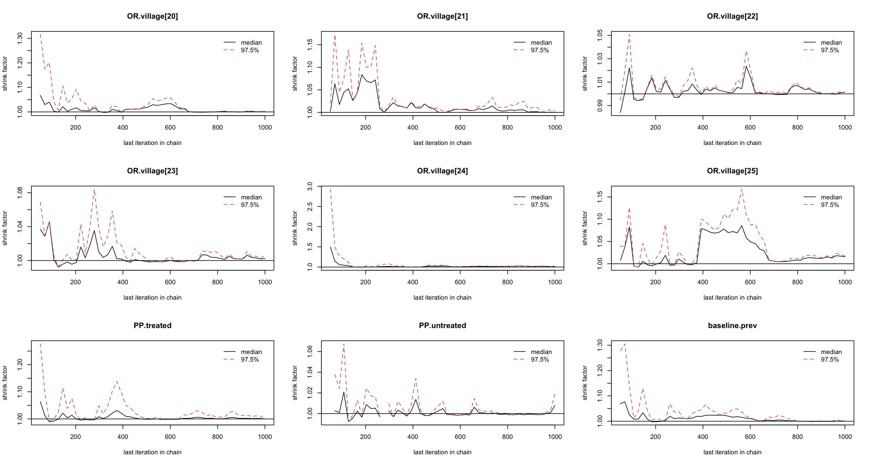
圖 102.14: Gelman-Rubin convergence statistic of parameters for GLM about the odds of malaria regarding netbeds use in Gambia children.
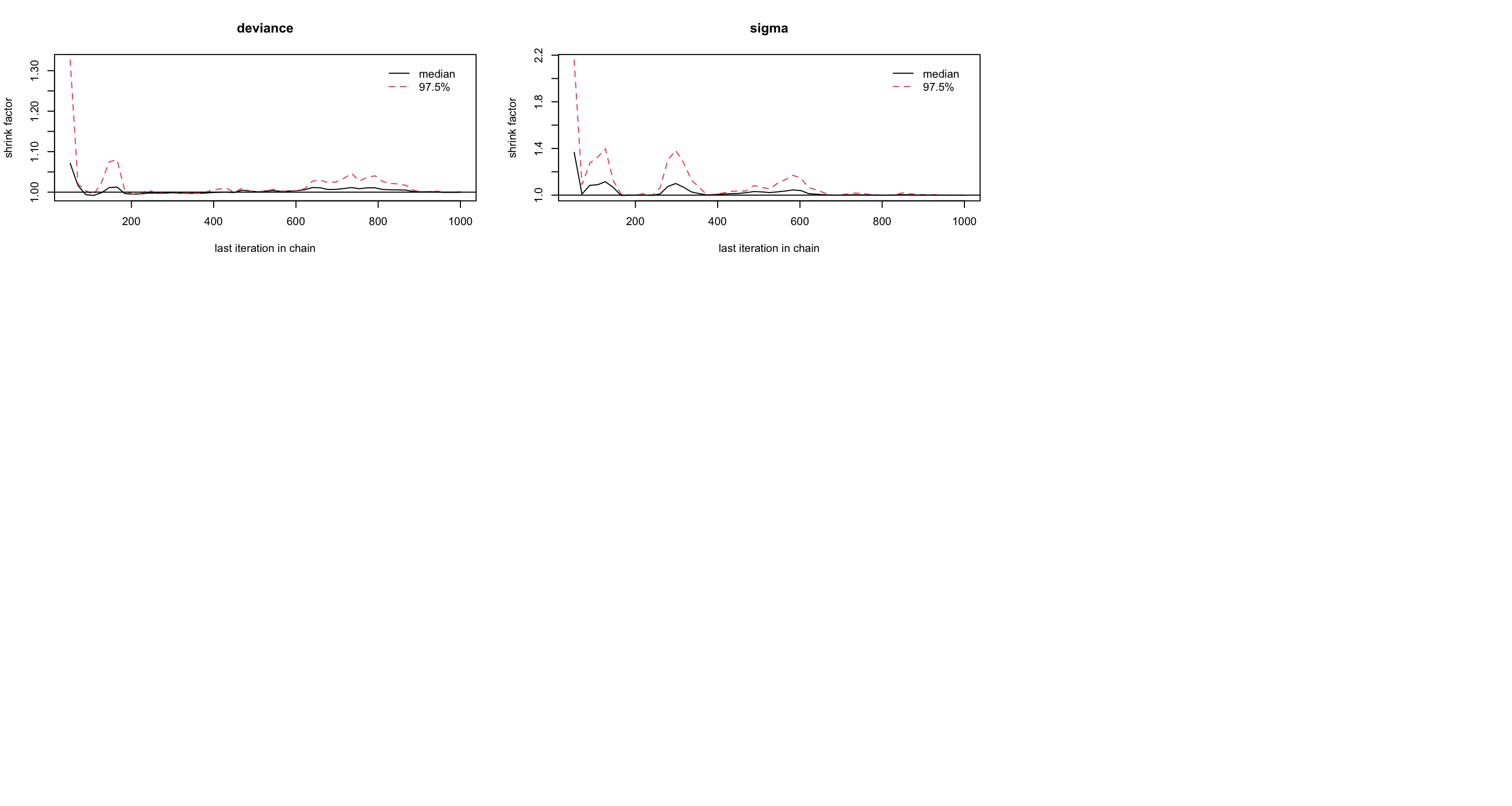
圖 102.15: Gelman-Rubin convergence statistic of parameters for GLM about the odds of malaria regarding netbeds use in Gambia children.
基本可以認爲刨除前1000次取樣 (burn-in) 可以達到收斂。
jagsModel <- jags(data = Dat,
                  model.file = paste(bugpath,
                                  "/backupfiles/malaria-model-hierarchical.txt",
                                  sep = ""),
                    parameters.to.save = parameters,
                     n.iter = 26000,
                     n.chains = 2,
                     inits = inits,
                     n.burnin = 1000,
                     n.thin = 1,
                    progress.bar = "none")
## Compiling model graph
## Resolving undeclared variables
## Allocating nodes
## Graph information:
## Observed stochastic nodes: 149
## Unobserved stochastic nodes: 34
## Total graph size: 1435
##
## Initializing model## Inference for Bugs model at "/Users/chaoimacmini/Downloads/LSHTMlearningnote/backupfiles/malaria-model-hierarchical.txt", fit using jags,
## 2 chains, each with 26000 iterations (first 1000 discarded)
## n.sims = 50000 iterations saved
## mu.vect sd.vect 2.5% 25% 50% 75% 97.5% Rhat n.eff
## OR.age[2] 1.799 0.440 1.089 1.484 1.749 2.057 2.810 1.001 50000
## OR.age[3] 2.283 0.550 1.404 1.892 2.216 2.602 3.524 1.001 50000
## OR.age[4] 2.359 0.575 1.431 1.953 2.290 2.691 3.676 1.001 50000
## OR.bednet[2] 0.731 0.212 0.404 0.580 0.700 0.850 1.225 1.001 22000
## OR.bednet[3] 0.644 0.247 0.291 0.469 0.601 0.771 1.244 1.001 50000
## OR.bednet[4] 0.917 0.352 0.421 0.667 0.856 1.096 1.770 1.001 50000
## OR.green 0.954 0.062 0.835 0.912 0.953 0.993 1.082 1.001 50000
## OR.phc 0.697 0.337 0.254 0.469 0.631 0.845 1.528 1.001 50000
## OR.village[1] 2.739 1.309 1.059 1.842 2.462 3.322 6.002 1.001 50000
## OR.village[2] 1.255 0.507 0.543 0.901 1.163 1.510 2.480 1.001 28000
## OR.village[3] 1.379 0.786 0.436 0.848 1.200 1.696 3.383 1.001 34000
## OR.village[4] 0.782 0.410 0.258 0.505 0.698 0.963 1.787 1.001 50000
## OR.village[5] 1.333 0.682 0.465 0.867 1.189 1.631 3.026 1.001 17000
## OR.village[6] 1.094 0.598 0.350 0.687 0.962 1.351 2.615 1.001 50000
## OR.village[7] 3.307 1.620 1.269 2.209 2.958 4.012 7.341 1.001 50000
## OR.village[8] 0.481 0.224 0.173 0.324 0.441 0.588 1.031 1.001 11000
## OR.village[9] 0.237 0.119 0.077 0.153 0.214 0.295 0.529 1.001 50000
## OR.village[10] 1.086 0.552 0.376 0.706 0.971 1.338 2.474 1.001 50000
## OR.village[11] 0.734 0.446 0.196 0.432 0.633 0.918 1.853 1.001 50000
## OR.village[12] 2.040 0.979 0.760 1.364 1.839 2.484 4.484 1.001 50000
## OR.village[13] 1.831 1.648 0.333 0.878 1.410 2.245 5.926 1.001 50000
## OR.village[14] 0.730 0.400 0.217 0.454 0.646 0.909 1.724 1.001 50000
## OR.village[15] 0.341 0.206 0.093 0.201 0.297 0.428 0.851 1.001 29000
## OR.village[16] 0.666 0.351 0.206 0.421 0.596 0.831 1.544 1.001 9000
## OR.village[17] 1.312 0.675 0.446 0.844 1.171 1.613 3.032 1.001 12000
## OR.village[18] 4.373 2.513 1.464 2.691 3.771 5.341 10.921 1.001 50000
## OR.village[19] 0.919 0.478 0.303 0.588 0.821 1.134 2.129 1.001 50000
## OR.village[20] 1.334 0.661 0.483 0.882 1.199 1.627 2.977 1.001 50000
## OR.village[21] 2.753 1.365 1.029 1.827 2.466 3.340 6.196 1.001 50000
## OR.village[22] 1.093 0.548 0.390 0.719 0.979 1.339 2.443 1.001 50000
## OR.village[23] 1.174 0.571 0.425 0.779 1.057 1.436 2.586 1.001 50000
## OR.village[24] 0.393 0.301 0.068 0.195 0.317 0.502 1.162 1.001 21000
## OR.village[25] 2.547 1.503 0.818 1.564 2.204 3.112 6.335 1.001 50000
## PP.treated 0.664 0.472 0.000 0.000 1.000 1.000 1.000 1.001 9600
## PP.untreated 0.892 0.310 0.000 1.000 1.000 1.000 1.000 1.001 14000
## baseline.prev 0.321 0.086 0.171 0.260 0.316 0.376 0.507 1.001 50000
## sigma 0.921 0.195 0.609 0.785 0.898 1.030 1.363 1.001 50000
## deviance 367.626 7.526 354.810 362.269 367.018 372.225 384.025 1.001 50000
##
## For each parameter, n.eff is a crude measure of effective sample size,
## and Rhat is the potential scale reduction factor (at convergence, Rhat=1).
##
## DIC info (using the rule, pD = var(deviance)/2)
## pD = 28.3 and DIC = 395.9
## DIC is an estimate of expected predictive error (lower deviance is better).從多層邏輯回歸分析的結果來看,每個變量的事後概率分佈的標準差都比無考慮村莊這一隨機效應時要大一些。這主要是因爲,多層回歸模型考慮了數據中村莊這個層面的過度離散效應(overdispersion)。但是整體的來說,每個比值比的含義並沒有發生太多改變。另外,村莊層級的隨機效應,其方差的事後均值爲 0.915,這是相對高的過度離散效應的表現。DIC結果也比無隨機效應的邏輯回歸模型提升顯著 476.8->396.8。這也是村莊層級隨機效應十分顯著的證據之一。