第 51 章 交互作用 it’s all about interaction
51.1 設計一個交互作用模型
From Page 241 of the rethinking book:
We could cheat by splitting the data into two data frames. But it’s not a good idea to split the data in this way. Here are four reasons.
First, there are usually some parameters, such as \(\sigma\), that the model says do not depend in any way upon continent (the variable you want to split the data on). By splitting the data table, you are hurting the accuracy of the estimates of pooling all of the eivdence into one estimate. In effect, you have accidentally assumed that variance differs between African and non-African nations. Now, there is nothing wrong with that sort of assumption. But you want to avoid accidental assumptions.
Second …
Third, we may want to use information criteria or another method to compare models. In order to compare a model that treats all continents the same way to a model that allows different slopes in different continents, we need models that use all of the same data. This means that we cannot split the data for two separate models. We have to let a single model internally split the data.
Fourth, once you begin using multilevel models, you’ll see that there are advantages to borrowing information across categories like “Africa” and “not Africa.” This is especially true when sample sizes vary across categories, such that overfitting risk is higher within some categories. In other words, what we learn about ruggedness outside of Africa should have some effect on our estimate within Africa, and vise versa. Mulitlevel models borrow information in this way, in order to improve estimates in all categories. When we split the data, this borrowing is impossible.
51.1.1 設計非洲大陸地形的模型
我們先設計一個不包含是否是非洲大陸這一變量的模型。
data("rugged")
d <- rugged

# make log version of outcome
d$log_gdp <- log( d$rgdppc_2000 )

# extract countries with GDP data
dd <- d[ complete.cases( d$rgdppc_2000 ), ]

# rescale variables
dd$log_gdp_std <- dd$log_gdp / mean( dd$log_gdp )
dd$rugged_std <- dd$rugged / max( dd$rugged )
使用簡單線性回歸來分析土地的崎嶇程度和該地區的生產總值之間可能存在的關係:
\[ \begin{aligned} \log (y_i) & \sim \text{Normal}(\mu_i, \sigma) \\ \mu_i & = \alpha + \beta(r_i - \bar{r}) \end{aligned} \]
其中,
- \(y_i\) 是第 \(i\) 地區的GDP;
- \(r_i\) 是第 \(i\) 地區的崎嶇程度;
- \(\bar{r}\) 是全體地區崎嶇程度的平均值,大約是 0.215。
我們現在對與這兩者之間的關係並不瞭解,只能猜測,並賦予先驗概率分佈進行估算:
\[ \begin{aligned} \alpha & \sim \text{Normal}(1,1) \\ \beta & \sim \text{Normal}(0, 1) \\ \sigma & \sim \exp(1) \end{aligned} \]
把這些翻譯成R語言模型:
m8.1 <- quap(
  alist(
    log_gdp_std ~ dnorm( mu, sigma ),
    mu <- a + b * (rugged_std - 0.215),
    a ~ dnorm( 1, 1 ),
    b ~ dnorm( 0, 1 ),
    sigma ~ dexp(1)
  ), data = dd
)
讓我們先來審視一下我們選擇的先驗概率大致是什麼樣的:
set.seed(7)
prior <- extract.prior( m8.1 )

# set up the plot dimensions

plot(NULL, xlim = c(0, 1), ylim = c(0.5, 1.4),
     xlab = "ruggedness", ylab = "log GDP",
     bty = "n",
     main = "a ~ dnorm(1,1)\nb ~ dnorm(0,1)")
abline(h = min(dd$log_gdp_std), lty = 2)
abline(h = max(dd$log_gdp_std), lty = 2)
with(dd, abline(a = 1.28, b = -0.6,
       lty = 1, lwd = 1.5, col = c("blue")))

# draw 50 lines from the prior
rugged_seq <- seq(from = -0.1, to = 1.1, length.out = 30)
mu <- link( m8.1, post = prior, data = data.frame(rugged_std = rugged_seq))
for( i in 1:50 ) lines( rugged_seq, mu[i,], col = col.alpha("black", 0.3))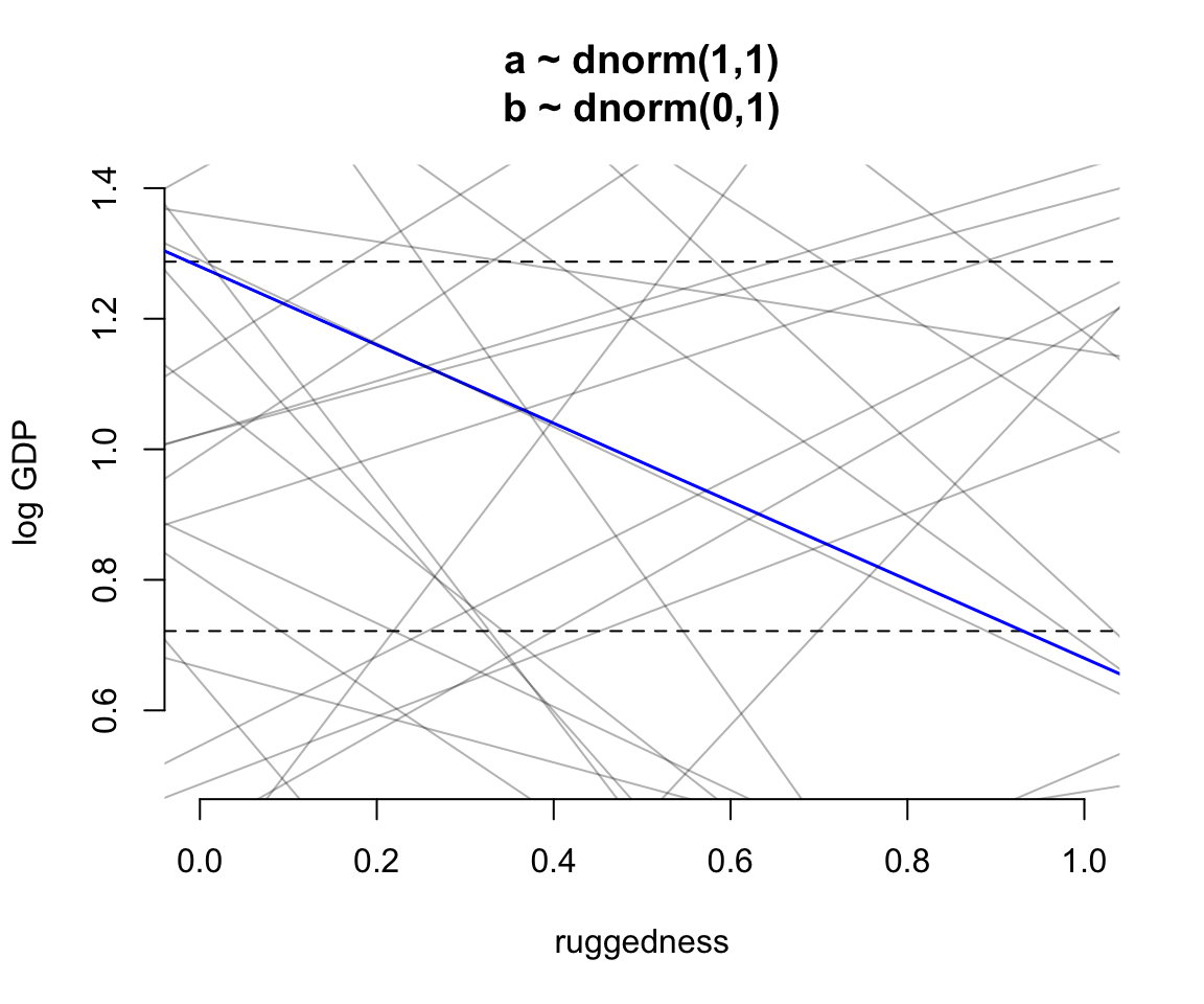
圖 51.1: Simulating in search of reasonable priors for the terrain ruggedness example. The dashed horizontal lines indicate the minimum and maximum observed GDP values. The first guess with very vague priors.
圖 51.1 中的上下兩條水平虛線分別是對數GDP的最大值和最小值。可以看見,我們這裏選擇使用的斜率和截距的先驗概率分佈是五花八門的,有正有負,有大有小,包含了很多令人匪夷所思的斜率或者截距。很顯然,我們最好對這些過於寬泛的斜率截距的選擇加以合理的限制以提高效率。例如選擇一個均值爲0,標準差是 0.1 的正(常)態分佈作爲截距 \(\alpha\) 的先驗概率分佈可能會比較合理。因爲 \(\text{Normal}(1, 0.1)\) 其實包含的意思是「我們認爲有95%的可能性截距是在 0.8-1.2之間」。同時,該圖 51.1 所示的斜率太過分散,有很多甚至比觀察數據給出的最大斜率 1.3 - 0.7 = 0.6 (藍色的線) 更加極端的斜率。在這裏使用的先驗概率中 \(\beta \sim \text{Normal}(0,1)\) ,有超過一半以上的斜率其實是要大於0.6的:
## [1] 0.545如果把斜率的先驗概率調整爲 \(\beta \sim \text{Normal}(0, 0.3)\) 的話,就能把斜率大於0.6的可能性降低到兩個標準差之外。
m8.1 <- quap(
  alist(
    log_gdp_std ~ dnorm( mu, sigma ),
    mu <- a + b * (rugged_std - 0.215),
    a ~ dnorm( 1, 0.1 ),
    b ~ dnorm( 0, 0.3 ),
    sigma ~ dexp(1)
  ), data = dd
)
set.seed(7)
prior <- extract.prior( m8.1 )

# set up the plot dimensions

plot(NULL, xlim = c(0, 1), ylim = c(0.5, 1.4),
     xlab = "ruggedness", ylab = "log GDP",
     bty = "n",
     main = "a ~ dnorm(1,1)\nb ~ dnorm(0,1)")
abline(h = min(dd$log_gdp_std), lty = 2)
abline(h = max(dd$log_gdp_std), lty = 2)
with(dd, abline(a = 1.28, b = -0.6,
       lty = 1, lwd = 1.5, col = c("blue")))

# draw 50 lines from the prior
rugged_seq <- seq(from = -0.1, to = 1.1, length.out = 30)
mu <- link( m8.1, post = prior, data = data.frame(rugged_std = rugged_seq))
for( i in 1:50 ) lines( rugged_seq, mu[i,], col = col.alpha("black", 0.3))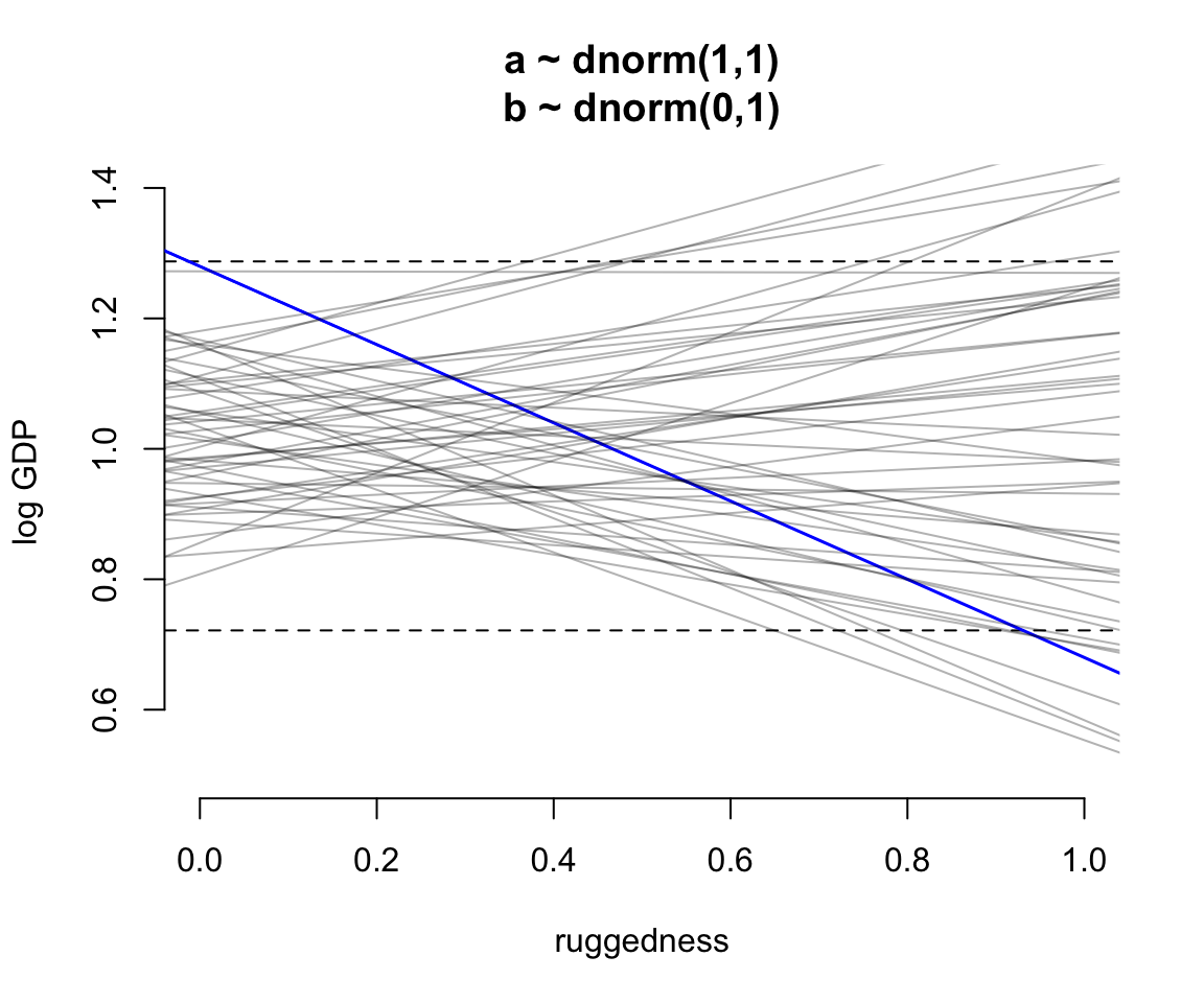
圖 51.2: Simulating in search of reasonable priors for the terrain ruggedness example. The dashed horizontal lines indicate the minimum and maximum observed GDP values. The improved model with much more plausible priors.
現在可以看看給出的事後概率分佈:
##               mean           sd         5.5%       94.5%
## a     0.9999995152 0.0104119724  0.983359172 1.016639858
## b     0.0019909345 0.0547934637 -0.085579603 0.089561472
## sigma 0.1364974025 0.0073961522  0.124676923 0.148317882
所以其實這裏我們給出的斜率的事後均值是零。那麼地區地理狀況是否崎嶇,和GDP之間真的沒有關係了嗎?
51.1.2 加一個指示變量並不是一個好選擇
最常見的增加非洲大陸這個變量的方法就是加一個指示變量:
\[ \mu_i = \alpha + \beta(r_i - \bar{r}) + \gamma A_i \]
其中,增加的變量 \(A_i\) 就是一個是否是非洲大陸國家的指示變量 (indicator variable)。但是事實上,每次增加一個這樣的指示變量時,你需要增加一個先驗概率給它的回歸係數。如此一來,它的副作用之一是告訴模型,我們對於在非洲大陸的國家的GDP的平均值有跟多的不確定性 (what the prior will necessarily do is tell the model that \(\mu_i\) for a nation in Africa is more uncertain, before seeing the data, than \(\mu_i\) outside Africa),這其實不是我們希望的額外假設,也沒有實際意義。
所以值得推薦的處理方法應該是使用索引變量 (index variable) 的方法使屬於非洲大陸或者之外的國家擁有不同的截距:
\[ \mu_i = \alpha_{\text{CID}[i]} + \beta(r_i - \bar{r}) \]
其中,\(\text{CID}[i]\) 就是這個索引變量,它取1時,截距就是非洲大陸國家的截距,它取2時,截距就是非洲大陸意外國家的截距。在 R 裏面很容易製作這樣的索引變量:
如此,就可以巧妙地避免了增加指示變量造成的額外先驗概率帶來的不確定性假設:
m8.2 <- quap(
  alist(
    log_gdp_std ~ dnorm(mu, sigma),
    mu <- a[cid] + b * ( rugged_std - 0.215 ),
    a[cid] ~ dnorm( 1, 0.1 ),
    b ~ dnorm( 0, 0.3 ),
    sigma ~ dexp(1)
  ), data = dd
)
precis(m8.2, depth = 2)
## mean sd 5.5% 94.5%
## a[1] 0.880412839 0.0159370032 0.85494243 0.905883248
## a[2] 1.049164255 0.0101855539 1.03288577 1.065442737
## b -0.046513472 0.0456867247 -0.11952968 0.026502738
## sigma 0.112387378 0.0060910769 0.10265266 0.122122095## WAIC SE dWAIC dSE pWAIC weight
## m8.2 -252.26868 15.305177 0.000000 NA 4.2585172 1.0000000e+00
## m8.1 -188.75420 13.292948 63.514478 15.146777 2.6904006 1.6143819e-14可以看到,a[1] 是非洲大陸國家的事後截距均值。可以看到它明顯是低於非洲大陸意外國家的事後截距均值 a[2]。對兩者的事後比較估算可以給我們更加確定的結果:
##          5%         94%
## -0.19901182 -0.13784897
可見兩類國家的GDP截距差很穩定地低於0。
rugged.seq <- seq(from  = -0.1, to = 1.1, length.out = 30)
# compute mu over samplesm fixing cid = 2 and then cid = 1
mu.NotAfrica <- link(m8.2,
                     data = data.frame(cid = 2, rugged_std = rugged.seq))
mu.Africa <- link(m8.2,
                  data = data.frame(cid = 1, rugged_std = rugged.seq))

# summarize to means and intervals
mu.NotAfrica_mu <- apply( mu.NotAfrica, 2, mean )
mu.NotAfrica_ci <- apply( mu.NotAfrica, 2, PI, prob = 0.97)
mu.Africa_mu <- apply( mu.Africa, 2, mean )
mu.Africa_ci <- apply( mu.Africa, 2, PI, prob = 0.97)

with(dd, plot(rugged_std[cid == 2], log_gdp_std[cid == 2], col=c("black"),
                    xlim = c(-0.05, 1.05), ylim = c(0.7, 1.3),
                    bty  = "n",
                    main = "m8.4",
                    xlab = "ruggedness (standardized)",
                    ylab = "log GDP (as proportion of mean)"))
with(dd, points(rugged_std[cid == 1],
       log_gdp_std[cid == 1],
       col = rangi2,
       pch = 16))
lines(rugged.seq, mu.NotAfrica_mu, lwd = 2)
lines(rugged.seq, mu.Africa_mu, lwd = 2, col = rangi2)
shade(mu.NotAfrica_ci, rugged.seq)
shade(mu.Africa_ci, rugged.seq, col = col.alpha(rangi2, 0.4))
text(0.9, 1.05, "Not Africa")
text(0.85, 0.9, "Africa", col = rangi2)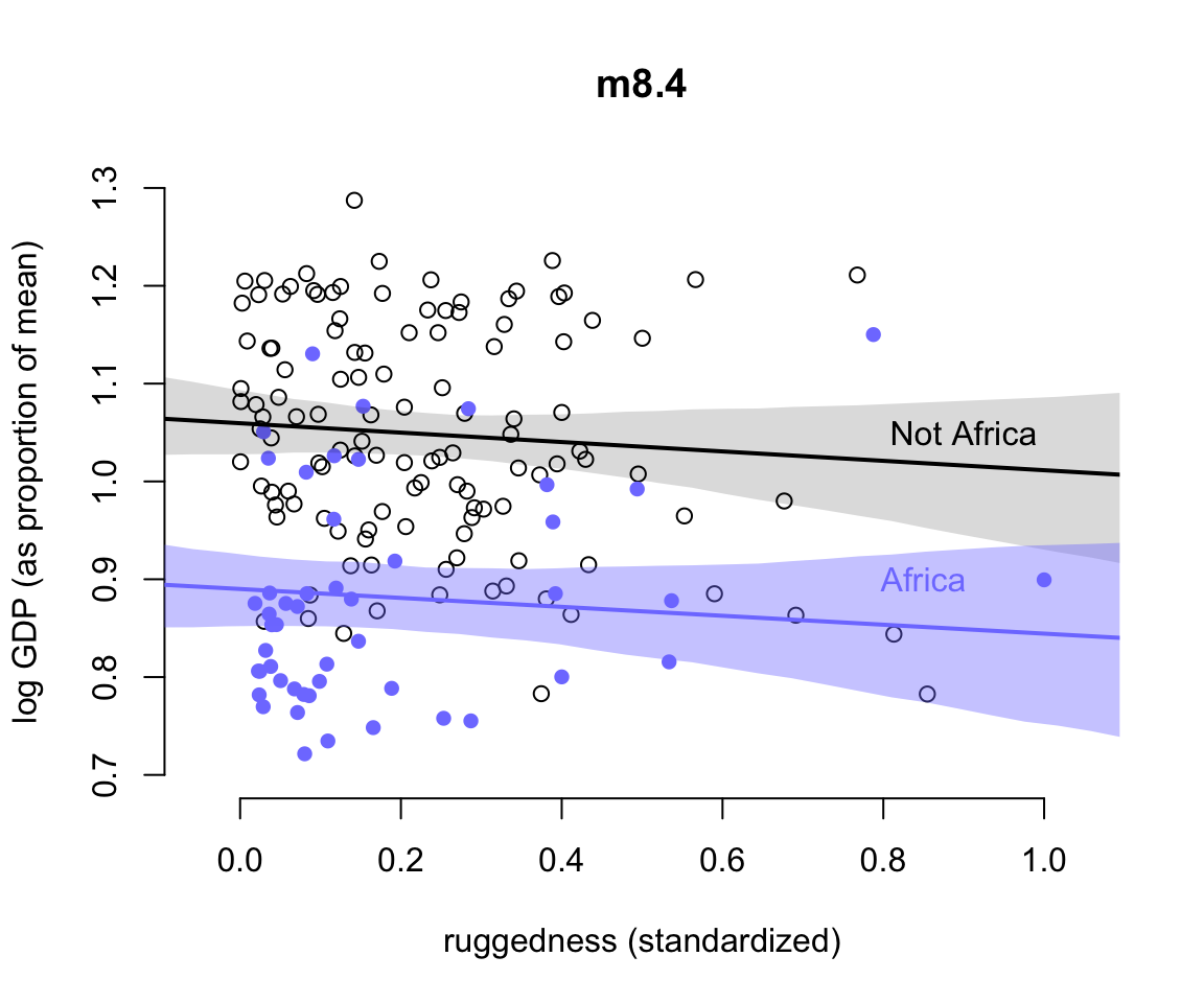
圖 51.3: Including an indicator for African nations has no effect on the slope. Africa nations are shown in blue. Non African nations are shown in black. Regression means for each subset of nations are shown in corresponding colors, along with 97% intervals shown by shading.
51.1.3 增加交互作用項是有幫助的
使用了索引變量的方法之後,我們發現加交互作用項,且避免增加冗餘的回歸係數的方法變得十分簡單:
\[ \mu_i = \alpha_{\text{CID}[i]} + \beta_{\text{CID}[i]}(r_i- \bar{r}) \]
m8.3 <- quap(
  alist(
    log_gdp_std ~ dnorm(mu, sigma),
    mu <- a[cid] + b[cid] * ( rugged_std - 0.215 ),
    a[cid] ~ dnorm( 1, 0.1 ),
    b[cid] ~ dnorm( 0, 0.3 ),
    sigma ~ dexp(1)
  ), data = dd
)
precis(m8.3, depth = 2)
## mean sd 5.5% 94.5%
## a[1] 0.88654416 0.0156763781 0.861490280 0.91159804
## a[2] 1.05056894 0.0099370706 1.034687582 1.06645030
## b[1] 0.13261316 0.0742076292 0.014015041 0.25121129
## b[2] -0.14272534 0.0547517457 -0.230229209 -0.05522148
## sigma 0.10949928 0.0059359892 0.100012419 0.11898613此時我們發現除了截距在非洲與非洲之外國家之間並不相同,他們和地區GDP之間的關係的斜率竟然也是相反的。比較這三個模型的模型指標:
##            WAIC        SE     dWAIC        dSE     pWAIC        weight
## m8.3 -259.31316 15.151912  0.000000         NA 5.0758988 9.7283924e-01
## m8.2 -252.15627 15.336212  7.156891  6.6853645 4.2959011 2.7160762e-02
## m8.1 -188.63140 13.331628 70.681757 15.4350065 2.7323144 4.3620684e-16
51.1.4 繪製交叉作用
- 非洲國家的GDP和其地理崎嶇程度之間的關係圖:
# Plot Africa - cid = 1
d.A1 <- dd[dd$cid == 1,]
plot(d.A1$rugged_std, d.A1$log_gdp_std, pch = 16,
     col = rangi2,
     bty = "n",
     main = "African nations",
     xlab = "ruggedness (standardized)",
     ylab = "log GDP (as proportion of mean)",
     xlim = c(0,1))
mu <- link( m8.3, data = data.frame( cid = 1, rugged_std = rugged_seq))
mu_mean <- apply( mu, 2, mean )
mu_ci <- apply( mu, 2, PI, prob = 0.97)
lines( rugged_seq, mu_mean, lwd = 2)
shade(mu_ci, rugged_seq, col = col.alpha(rangi2, 0.3))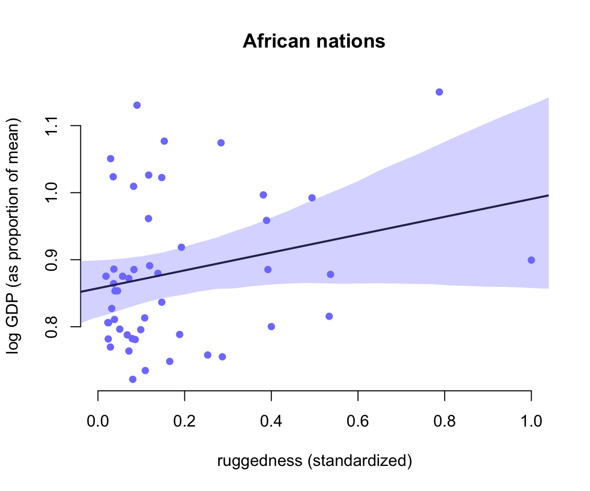
圖 51.4: Posterior predictitions for the terrain ruggedness model, including the interaction between Africa and ruggedness. Shaded regions are 97% posterior intervals of the mean. (Countries within Africa)
- 非洲大陸意外國家的GDP和其地理崎嶇程度之間的關係圖:
# plot non-Africa - cid = 2

d.A2 <- dd[dd$cid == 2,]
plot(d.A2$rugged_std, d.A2$log_gdp_std, pch = 1,
     col = "black",
     bty = "n",
     main = "Non-African nations",
     xlab = "ruggedness (standardized)",
     ylab = "log GDP (as proportion of mean)",
     xlim = c(0,1))
mu <- link( m8.3, data = data.frame( cid = 2, rugged_std = rugged_seq))
mu_mean <- apply( mu, 2, mean )
mu_ci <- apply( mu, 2, PI, prob = 0.97)
lines( rugged_seq, mu_mean, lwd = 2)
shade(mu_ci, rugged_seq)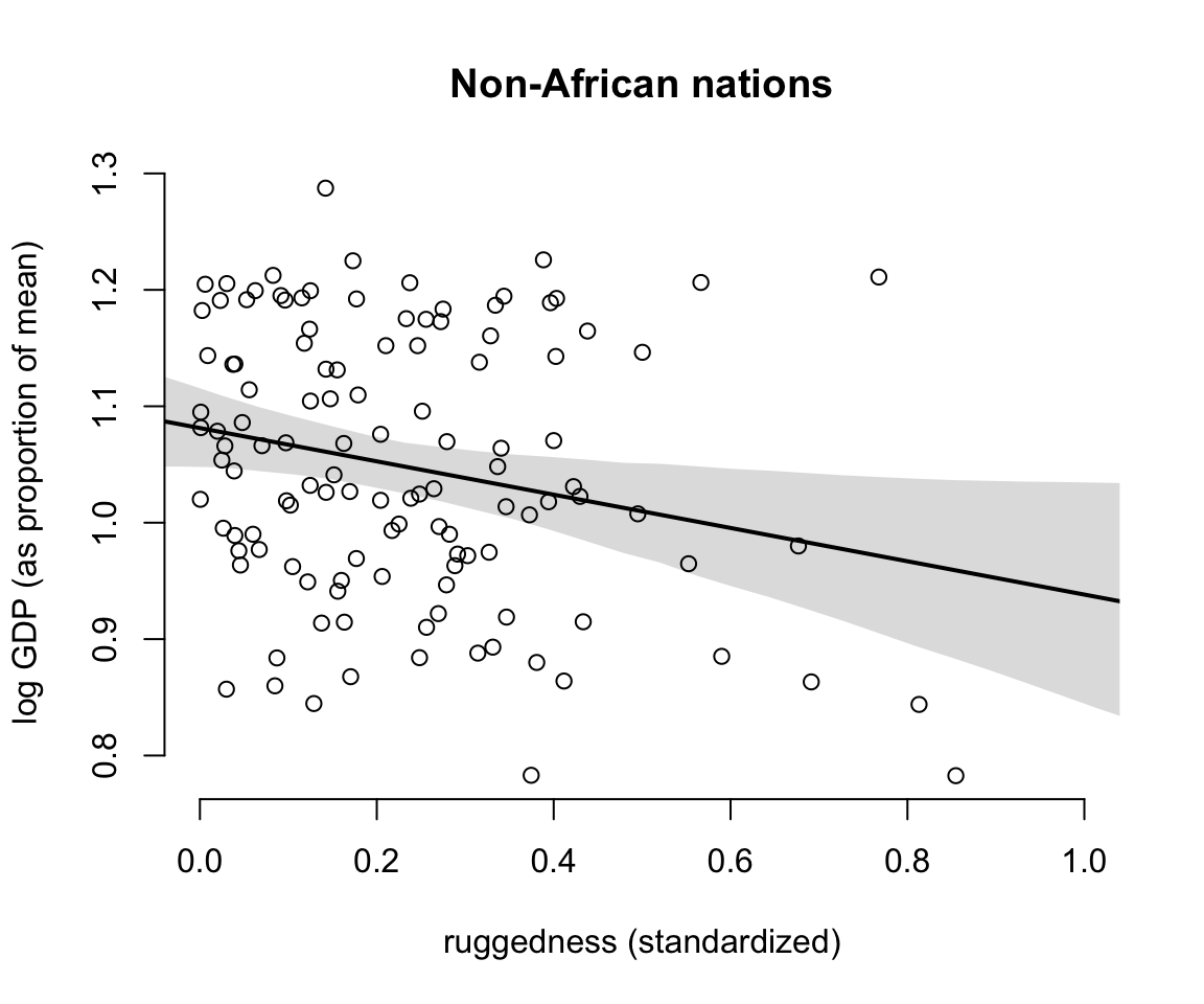
圖 51.5: Posterior predictitions for the terrain ruggedness model, including the interaction between Africa and ruggedness. Shaded regions are 97% posterior intervals of the mean. (Countries outside of Africa)
51.2 連續型變量之間的交互作用
51.2.1 Winter flower 冬天的花
數據是來自測量鬱金香在不同的種植環境條件下的開花尺寸。
## 'data.frame':    27 obs. of  4 variables:
##  $ bed   : Factor w/ 3 levels "a","b","c": 1 1 1 1 1 1 1 1 1 2 ...
##  $ water : int  1 1 1 2 2 2 3 3 3 1 ...
##  $ shade : int  1 2 3 1 2 3 1 2 3 1 ...
##  $ blooms: num  0 0 111 183.5 59.2 ...
其中,結果變量是 blooms ,預測變量使用 water, shade 。我們很容易理解因爲水和陽光是影響植物開花的重要條件。但我們還是對這兩個變量之間是不是有交互作用感興趣。因爲沒有水光有陽光,或者只有陽光沒有水,對植物的生長都沒有好處。
我們使用兩個模型,
- 包含水和陽光的兩個變量,沒有交互作用項
- 包含水和陽光的兩個變量,同時包括交互作用項
沒有交互作用的模型:
\[ \begin{aligned} B_i & \sim \text{Normal}(\mu_i, \sigma) \\ \mu_i & = \alpha + \beta_w(W_i - \bar{W}) + \beta_S(S_i - \bar{S}) \end{aligned} \]
爲了是估計過程更加順利,我們把 \(W,S\) 中心化(範圍控制在-1~1之間),把 \(B\) 轉換成一個相對其最大值的比例的變量,也就是範圍控制在 0~1 之間:
d$blooms_std <- d$blooms / max(d$blooms)
d$water_cent <- d$water - mean(d$water)
d$shade_cent <- d$shade - mean(d$shade)

precis(d, prob = 1)
## mean sd 0% 100% histogram
## bed NaN NA NA NA
## water 2.00000000 0.83205029 1 3.00 ▇▁▁▁▇▁▁▁▁▇
## shade 2.00000000 0.83205029 1 3.00 ▇▁▁▁▇▁▁▁▁▇
## blooms 128.99370370 92.68392285 0 361.66 ▅▇▇▂▃▁▁▁
## blooms_std 0.35667119 0.25627364 0 1.00 ▅▃▇▇▁▃▃▁▁▁
## water_cent 0.00000000 0.83205029 -1 1.00 ▇▁▁▁▇▁▁▁▁▇
## shade_cent 0.00000000 0.83205029 -1 1.00 ▇▁▁▁▇▁▁▁▁▇之所以在這裏給 blooms 修改尺度的最主要理由是,它的原始尺寸會導致模型擬合較爲困難,其二,修改了尺寸之後有助於我們選擇合理的先驗概率分佈。這裏先對三個參數的先驗概率分佈做一個最初步的猜想:
\[ \begin{aligned} \alpha & \sim \text{Normal}(0.5, 1) \\ \beta_W & \sim \text{Normal}(0,1) \\ \beta_S & \sim \text{Normal}(0,1) \end{aligned} \]
這裏使用均值 0.5 給截距 \(\alpha\) 是因爲我們初步認爲當水和陽光處於其本身的均值時,我們期待開花的大小應該是在觀測值中最大的尺寸的一半左右。兩個斜率的先驗概率的均值是0,表示我們不認爲有哪些有用的信息提示這兩個斜率究竟是正還是負。
但是,截距 \(\alpha\) 的實際可能取值範圍是在 (0,1) 之間,但是如果我們使用 \(\alpha \sim \text{Normal}(0.5, 1)\) 的話,表示有許多潛在的截距是在我們認爲合理範圍之外的:
## [1] 0.6215把標準差修改成爲 0.25 應該就能把不合理的截距取值限制在 5% 可能性以下:
## [1] 0.0434相似地,我們也需要控制兩個斜率的先驗概率分佈的標準差,使得結果變量的取值在合理範圍內:
m8.4 <- quap(
  alist(
    blooms_std ~ dnorm( mu, sigma),
    mu <- a + bw * water_cent + bs * shade_cent,
    a ~ dnorm( 0.5, 0.25 ),
    bw ~ dnorm( 0, 0.25 ),
    bs ~ dnorm( 0, 0.25 ),
    sigma ~ dexp(1)
  ), data = d
)
precis(m8.4)
## mean sd 5.5% 94.5%
## a 0.35877210 0.030216466 0.31048035 0.407063847
## bw 0.20503592 0.036886543 0.14608410 0.263987738
## bs -0.11253064 0.036872698 -0.17146034 -0.053600951
## sigma 0.15814122 0.021439313 0.12387706 0.192405381接下來,我們思考如何定義兩個連續型變量之間的交互作用。如何才能使一個模型滿足我們的假設,也就是,開花的大小尺寸同時收到陽光和水的影響?比如說,當水很少,增加陽光對於開花並沒有太多的好處這樣的觀察結果。這裏其實是在說,water 變量的回歸係數,\(\beta_W\) 是取決於陽光的。或者相似地,可以反過來思考,就是 shade 變量的回歸係數,\(\beta_S\) 是取決於水的。此時,我們似乎沒辦法沿用索引變量的方法。但是使用線性回歸模型的思考方式,我們可以解決這個難題,也就是給水的斜率和陽光之間也定義一個線性回歸函數:
\[ \begin{aligned} \mu_i & = \alpha + \gamma_{W,i} W_i + \beta_S S_i \\ \gamma_{W,i} & = \beta_W + \beta_{WS}S_i \end{aligned} \]
其中,
- \(\gamma_{W,i}\) 就是在第一個方程裏水本身的斜率。
- \(\beta_W\) 是當陽光是平均值時,陽光對水的斜率的影響。
- \(\beta_{WS}\) 就是隨着陽光改變而改變的水的斜率。
你可能更加常見的表達方式是:
\[ \begin{aligned} \mu_i & = \alpha + \underbrace{(\beta_W + \beta_{WS}S_i)}_{\gamma_{W,i}}W_i + \beta_S S_i \\ & = \alpha + \beta_W W_i + \beta_S S_i + \beta_{WS}S_iW_i \end{aligned} \]
那麼我們還需要別忘記給這個新增加的參數的回歸係數 \(\beta_{WS}\) 設計它的先驗概率分佈。
m8.5 <- quap(
  alist(
  blooms_std ~ dnorm( mu, sigma ),
  mu <- a + bw * water_cent + bs * shade_cent + bws * water_cent * shade_cent,
  a ~ dnorm( 0.5, 0.25 ),
  bw ~ dnorm( 0, 0.25 ),
  bs ~ dnorm( 0, 0.25 ),
  bws ~ dnorm( 0, 0.25 ),
  sigma ~ dexp(1)
  ), data = d
)
precis(m8.5)
## mean sd 5.5% 94.5%
## a 0.35798434 0.023918650 0.319757716 0.396210961
## bw 0.20673108 0.029234311 0.160009004 0.253453156
## bs -0.11346419 0.029227282 -0.160175032 -0.066753348
## bws -0.14315705 0.035679412 -0.200179645 -0.086134462
## sigma 0.12484398 0.016940114 0.097770408 0.15191755651.2.2 繪製事後預測圖
三聯畫 (triptych) 會是幫助我們理解連續變量之間交互作用的極佳示意圖。每個圖都需要能夠表達模型所預測的水與開花尺寸大小之間的關係,同時,每張圖會指定陽光爲某一個固定值,來看陽光,水,和開花尺寸三者之間的關係的變化。由於本例中,已知陽光(或者水)只有三個強度的取值:-1,0,1。所以三聯圖是首選。其他時候,如果是處理嚴格的連續變量的話,你完全可以選取三個代表性的取值,如最低值,中位數,和最大值來繪製三聯圖。
par(mfrow = c(1,3)) # 3 plots in a row

for (s in -1:1) {
  idx <- which( d$shade_cent == s)
  plot( d$water_cent[idx], d$blooms_std[idx],
        xlim = c(-1, 1),
        bty = "n",
        ylim = c(0, 1),
        main = paste("m8.4 (no interaction)\npost: shade = ", s),
        xlab = "water (centered)",
        ylab = "blooms (rescaled)",
        pch = 16,
        col = rangi2)
  mu <- link(m8.4, data = data.frame(shade_cent = s, water_cent = -1:1))
  for( i in 1:20 ) lines( -1:1, mu[i, ], col = col.alpha("black", 0.3))
}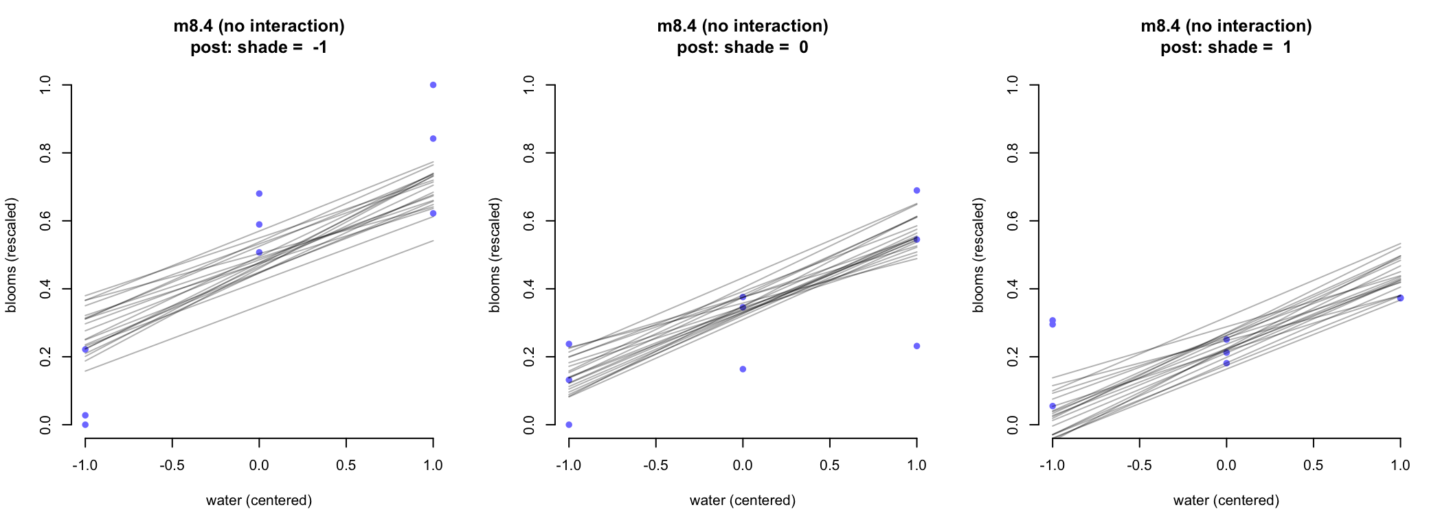
圖 51.6: Triptych plots of posterior predicted blooms across water and shade treatments. (without an interaction between water and shade)
圖 51.6 顯示的是沒有交互作用項時給出的事後預測直線。每個陽光,水條件下,水和開花尺寸之間關係的直線並沒有斜率上的顯著變化。給 m8.5 繪製相似的三聯圖,可以看出斜率隨着不同陽光強度發生了變化:
par(mfrow = c(1,3)) # 3 plots in a row

for (s in -1:1) {
  idx <- which( d$shade_cent == s)
  plot( d$water_cent[idx], d$blooms_std[idx],
        xlim = c(-1, 1),
        bty = "n",
        ylim = c(0, 1),
        main = paste("m8.5 (with interaction)\npost: shade = ", s),
        xlab = "water (centered)",
        ylab = "blooms (rescaled)",
        pch = 16,
        col = rangi2)
  mu <- link(m8.5, data = data.frame(shade_cent = s, water_cent = -1:1))
  for( i in 1:20 ) lines( -1:1, mu[i, ], col = col.alpha("black", 0.3))
}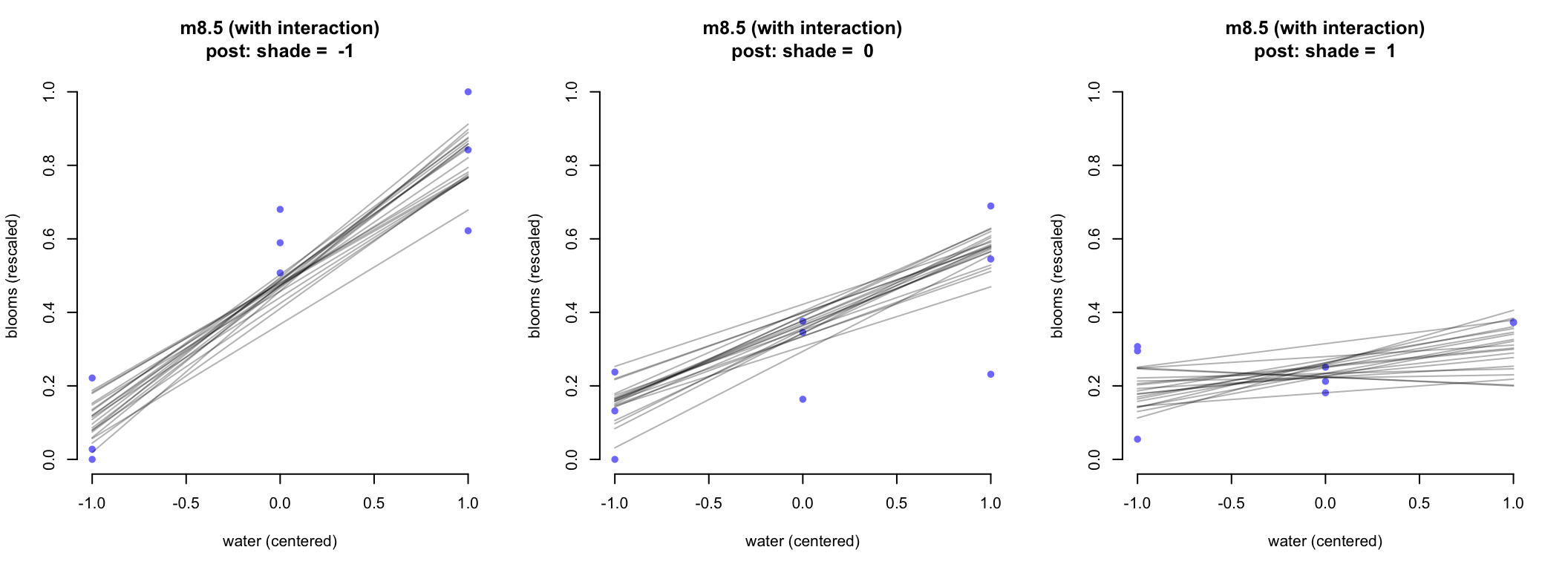
圖 51.7: Triptych plots of posterior predicted blooms across water and shade treatments. (with an interaction between water and shade)
很明顯,加入了交互作用之後的模型更加符合實際情況,圖 51.7 中不同強度陽光條件下,水和開花尺寸之間的關係的斜率發生了顯著的變化。當陽光不強時,水和開花尺寸之間的關係斜率較大,當陽光強度增加,這個斜率在下降。