第 58 章 廣義線性迴歸入門
線性迴歸方法是十分強大的建模工具,可惜的是它只能適用與因變量爲連續型變量的情況。廣義線性迴歸模型 (或者叫一般化線性迴歸模型 generalised linear models, GLM) 是一大類將線性迴歸模型拓展到因變量可以使用二進制,計數,分組型變量的建模工具。
58.1 指數分佈家族
一個服從正態分佈的隨機變量 \(Y\) 的概率密度方程 (probability density function, PDF) 可以寫作
\[ f(y) = \frac{1}{\sqrt{2\pi\sigma^2}}e^{-\frac{(y-\mu)^2}{2\sigma^2}} \]
給 PDF 的左右兩邊同時取自然底數的對數,方程變形爲
\[ \begin{aligned} \text{ln}\{f(y)\} & = -\frac{y^2}{2\sigma^2} + \frac{y\cdot\mu}{\sigma^2} - \frac{\mu^2}{2\sigma^2} -\frac{1}{2}\text{ln}(2\pi\sigma^2) \\ & = \frac{y\cdot\mu - \frac{\mu^2}{2}}{\sigma^2} - [\frac{y^2}{2\sigma^2} + \frac{1}{2}\text{ln}(2\pi\sigma^2) ] \end{aligned} \tag{58.1} \]
如果令
\[ \begin{aligned} \theta & = \mu \\ \psi & = \sigma^2 \\ b(\theta) & = \frac{\mu^2}{2} \\ c(y, \theta) & = \frac{y^2}{2\sigma^2} + \frac{1}{2}\text{ln}(2\pi\sigma^2) \end{aligned} \]
那麼上面的式子 (58.1) 可以被整理爲:
\[ \begin{equation} \text{ln}\{f(y)\} = \frac{y\cdot\theta - b(\theta)}{\psi} - c(y, \theta) \end{equation} \tag{58.2} \]
此處有重要結論: 凡是分佈的概率密度方程的對數方程能夠轉換整理成 (58.2) 形式的分佈,都隸屬於指數分佈家族 (the Exponential Family of distributions)。
58.1.1 泊松分佈和二項分佈的指數分佈家族屬性
- 泊松分佈 Poisson Distribution
\[ \begin{aligned} f(y) & = \text{Pr}(Y = y) = \frac{\mu^y e^{-\mu}}{y!}, y = 0,1,2,\cdots \\ \text{ln}\{ f(y) \} & = y\cdot\text{ln}(\mu) - \mu - \text{ln}(y!) \\ \text{Let } &\color{red}{\boxed{\theta = \text{ln}(\mu), \psi = 1, b(\theta) = \mu, c(y,\psi) = \text{ln}(y!)}} \\ \Rightarrow \text{ln}\{f(y)\} & = \frac{y\cdot\theta - b(\theta)}{\psi} - c(y, \theta) \\ \end{aligned} \]
所以,泊松分佈屬於指數分佈家族成員。
- 二項分佈 Binommial Distribution
\[ \begin{aligned} f(y) & = \text{Pr}(Y = y) = \binom{n}{y}\pi^y(1-\pi)^{n-y}, y = 0,1,2,\cdots\\ \text{ln}\{ f(y) \} & = y\cdot \text{ln}(\pi) + (n - y)\text{ln}(1-\pi) + \text{ln}\{\binom{n}{y}\} \\ & = y\cdot \text{ln}(\frac{\pi}{1-\pi}) + n\text{ln}(1-\pi) + \text{ln}\{\binom{n}{y}\} \\ \text{Let } &\color{red}{\boxed{\theta = \text{ln}(\frac{\pi}{1-\pi}), \psi = 1,}} \\ &\color{red}{\boxed{b(\theta) = -n\text{ln}(1-\pi), c(y, \psi) = -\text{ln}\{\binom{n}{y}\}}}\\ \Rightarrow \text{ln}\{f(y)\} & = \frac{y\cdot\theta - b(\theta)}{\psi} - c(y, \theta) \\ \end{aligned} \]
所以,二項分佈也屬於指數分佈家族成員。
指數分佈家族成員的數學表達式 (58.2) 中,
- \(\theta\) 被叫做標準 (或者叫自然) 參數 (canonical or natural parameter),相關的函數被叫做標準鏈接函數 (canonical link function),如上面所列舉的例子中:泊松分佈時用的對數函數 \(\text{ln}(\mu)\),二項分佈時用的邏輯函數 (logit function) \(\text{ln}(\frac{\pi}{1-\pi})\),鏈接函數可能還有別的選擇,(例如,二項分佈數據的另一種標準鏈接函數是概率函数 (probit function \(\Phi^{-1}(P)\))),同時它對於條件推斷 conditional inference 至關重要,因爲它還提示我們應該用什麼樣的算法去估計我們苦苦尋找的人羣參數。
- \(\phi\) 被命名爲尺度參數 (scale or dispersion parameter),泊松分佈和二項分佈的尺度參數是 \(1\)。但是正態分佈的尺度參數是方差 \(\sigma^2\),且常常是未知的,需要從樣本數據中估計。尺度參數是否需要從樣本中獲取其估計值,對於實際統計推斷或者假設檢驗的過程有重大影響。
廣義線性迴歸就是這個指數分佈家族數據共通的一種統計建模過程,所以,在這一“屋檐”下,它衍生出衆多種類的統計模型。
58.1.2 Exercise. Exponential distribution
證明指數分佈本身也屬於指數分佈家族,定義其標準鏈接函數和標準參數。
證明
\[ \begin{aligned} Y \sim \text{exp}(\lambda) & \rightarrow f(y) = \lambda \text{exp}(-y\lambda), y > 0\\ \Rightarrow \text{ln}\{ f(y) \} & = - y \lambda + \text{ln}(\lambda) \\ \text{Let } & \color{red}{\theta = -\lambda, b(\theta) = - \text{ln}(\lambda), \phi = 1, c(y, \phi) = 0} \\ \Rightarrow \text{ln}\{f(y)\} & = \frac{y\cdot\theta - b(\theta)}{\phi} - c(y, \theta) \\ \text{Because } E(Y) & = \frac{1}{\lambda}, \text{ the canonical link is } g(\lambda) = -\frac{1}{\lambda}\\ \end{aligned} \]
58.2 廣義線性迴歸模型之定義
一個四肢健全的廣義線性模型包括三個部分:
- 因變量分佈 (或者叫響應變量分佈,response distribution):\(Y_i, i = 1,\cdots,n\) 可以被認爲是互相獨立且服從指數家族分佈,設其期望值 (均值) \(E(Y_i) = \mu_i\);
- 線性預測方程 (linear predictor):預測變量及其各自的參數以線性迴歸形式進入模型,其中第 \(i\) 個觀測值的線性預測值爲:
\[\eta_i = \alpha + \beta_1 x_{i1} + \cdots + \beta_p x_{ip}\] - 鏈接函數 (link function):鏈接函數連接的是線性預測方程 \(\eta_i\) 和其期待值 (均值) 之間 \(\mu_i\) 的關係。
\[g(\mu_i) = \eta_i\]
簡單線性迴歸模型本身當然也數據廣義線性迴歸模型:
- 因變量分佈是正態分佈;
- 線性預測值也是線性迴歸形式;
- 鏈接函數是它因變量本身 (the identity function)。
58.3 注意
- 廣義線性迴歸的線性預測方程部分的意義,需要澄清的是它指的是 參數 parameter 之間呈線性關係,預測變量本身可以有二次方,三次方,多次方,因爲這些多項式線性迴歸本身仍然是線性的如: \[\eta_i = \alpha + \beta_1 x_i + \beta_2 x_i^2 + \cdots + \beta_p x_i^p\]
然而,這樣的形式 \[\eta_i = \alpha (1- e^{\beta_1 x_{i1}})\]
就不能說是一個線性預測方程。 - 除了有很少的特例。廣義線性迴歸擬合後的參數估計,推斷,模型評價和比較時使用的原理都一樣,不同的只有各自的分佈和鏈接函數。
- 通常選用的鏈接方程,要能夠使線性預測方程的取值範圍達到所有實數 \(-\infty,+\infty\)。
- “模型的似然函數 the log likelihood of the model”,只是我們偷懶縮短了原文 “在給定數據的前提下,當所有參數均爲 \(\text{MLE}\) 時模型的對數似然函數 (the log likelihood function of the model for the given data evaluated at the MLE’s of the parameters)”,就是對數似然函數的極大值的意思 (i.e. the maximum of the log likelihood function)。
- 從本節開始往後的章節中 “模型,model”,“廣義線性模型,generalized linear model”,和 “GLM” 將被視爲同義詞。
58.4 如何在 R 裏擬合 “GLM”
這裏討論用極大似然法擬合 “GLM” 模型的方法。前面一章節的複習也是在告訴我們,利用極大似然法簡單說就是找到模型參數,使得似然函數能夠取到極大值。對於線性迴歸來說, \(\text{MLE}\) 可以用一個封閉式函數來計算;但是廣義線性迴歸模型則必須使用迭代法計算 (iterative methods)。
在 R 裏面擬合廣義線性模型的命令及其格式是:
glm(response variable ~ explanatory variables to form linear predictor, family=name of distribution(link=link function), data=dataset)Tips: See help(glm) for other modeling options. See help(family) for other allowable link functions for each family.
下面的數據來自一個心理學臨牀實驗,比較的是和安慰劑組相比,注射嗎啡組,注射海洛因組對象的精神病檢測指數的前後變化。
Mental <- read.table("../backupfiles/MENTAL.DAT", header =  FALSE, sep ="", col.names = c("treatment", "Before", "After"))
Mental$treatment[Mental$treatment == 1] <- "placebo"
Mental$treatment[Mental$treatment == 2] <- "morphine"
Mental$treatment[Mental$treatment == 3] <- "heroin"
Mental$treatment <- factor(Mental$treatment, levels = c("placebo", "morphine", "heroin"))
head(Mental)
## treatment Before After
## 1 placebo 0 7
## 2 placebo 2 1
## 3 placebo 14 10
## 4 placebo 5 10
## 5 placebo 5 6
## 6 placebo 4 2我們來比較一下簡單線性迴歸的代碼輸出結果和廣義線性迴歸代碼輸出結果是否一致:
用 lm 命令,擬合因變量爲注射後精神病檢測指數,預測變量爲治療方式和注射錢精神病檢測指數,及兩者的交互作用項:
##
## Call:
## lm(formula = After ~ treatment * Before, data = Mental)
##
## Residuals:
##      Min       1Q   Median       3Q      Max
## -7.82808 -1.93513 -0.51606  1.41607 11.36012
##
## Coefficients:
##                           Estimate Std. Error t value Pr(>|t|)
## (Intercept)               1.978030   1.294069  1.5285 0.131158
## treatmentmorphine        -1.211742   1.750342 -0.6923 0.491185
## treatmentheroin          -1.461968   1.771855 -0.8251 0.412284
## Before                    0.593939   0.183468  3.2373 0.001889 **
## treatmentmorphine:Before -0.089526   0.248346 -0.3605 0.719633
## treatmentheroin:Before   -0.312985   0.250383 -1.2500 0.215704
## ---
## Signif. codes:  0 '***' 0.001 '**' 0.01 '*' 0.05 '.' 0.1 ' ' 1
##
## Residual standard error: 3.3329 on 66 degrees of freedom
## Multiple R-squared:  0.34418,    Adjusted R-squared:  0.29449
## F-statistic: 6.9274 on 5 and 66 DF,  p-value: 0.000029744
同樣的模型也可以用 glm 命令擬合:
Model2 <- glm(After ~ treatment*Before, family = gaussian(link = "identity"), data = Mental)
summary(Model2)
##
## Call:
## glm(formula = After ~ treatment * Before, family = gaussian(link = "identity"),
## data = Mental)
##
## Deviance Residuals:
## Min 1Q Median 3Q Max
## -7.82808 -1.93513 -0.51606 1.41607 11.36012
##
## Coefficients:
## Estimate Std. Error t value Pr(>|t|)
## (Intercept) 1.978030 1.294069 1.5285 0.131158
## treatmentmorphine -1.211742 1.750342 -0.6923 0.491185
## treatmentheroin -1.461968 1.771855 -0.8251 0.412284
## Before 0.593939 0.183468 3.2373 0.001889 **
## treatmentmorphine:Before -0.089526 0.248346 -0.3605 0.719633
## treatmentheroin:Before -0.312985 0.250383 -1.2500 0.215704
## ---
## Signif. codes: 0 '***' 0.001 '**' 0.01 '*' 0.05 '.' 0.1 ' ' 1
##
## (Dispersion parameter for gaussian family taken to be 11.107994)
##
## Null deviance: 1117.875 on 71 degrees of freedom
## Residual deviance: 733.128 on 66 degrees of freedom
## AIC: 385.414
##
## Number of Fisher Scoring iterations: 2可以看到,glm 命令的輸出結果略多,但是參數估計的部分是完全相同的。但是如果你用的是坑爹的 STATA,那裏面的 glm 命令中的統計檢驗量和 \(p\) 值用的則是正態分佈近似法。所以在 STATA 裏面簡單線性迴歸模型最好不要使用 glm 命令:
 glm After i.treatt##c.Before, family(gaussian) link(identity)

Iteration 0:   log likelihood = -185.70711

Generalized linear models                         No. of obs      =         72
Optimization     : ML                             Residual df     =         66
                                                  Scale parameter =   11.10799
Deviance         =  733.1276068                   (1/df) Deviance =   11.10799
Pearson          =  733.1276068                   (1/df) Pearson  =   11.10799

Variance function: V(u) = 1                       [Gaussian]
Link function    : g(u) = u                       [Identity]

                                                  AIC             =   5.325197
Log likelihood   =  -185.707106                   BIC             =   450.8676

------------------------------------------------------------------------------
             |                 OIM
        After|      Coef.   Std. Err.      z    P>|z|     [95% Conf. Interval]
-------------+----------------------------------------------------------------
       treat |
          2  |  -1.211742   1.750342    -0.69   0.489    -4.642349    2.218865
          3  |  -1.461968   1.771855    -0.83   0.409    -4.934741    2.010805
             |
      Before |   .5939394   .1834682     3.24   0.001     .2343483    .9535305
             |
 treat#Before|
          2  |  -.0895258   .2483459    -0.36   0.718    -.5762749    .3972233
          3  |  -.3129855   .2503829    -1.25   0.211     -.803727    .1777561
             |
       _cons |    1.97803   1.294069     1.53   0.126    -.5582981    4.514359
------------------------------------------------------------------------------
回到 R 來, 當儲存了一個 Model2 向量在 R 裏之後,你可以用下面的各種命令獲取你想要的各種有用的信息。
##                                2.5 %     97.5 %
## (Intercept)              -0.55829809 4.51435869
## treatmentmorphine        -4.64234925 2.21886536
## treatmentheroin          -4.93474055 2.01080452
## Before                    0.23434829 0.95353050
## treatmentmorphine:Before -0.57627487 0.39722332
## treatmentheroin:Before -0.80372697 0.17775605## (Intercept) treatmentmorphine treatmentheroin Before
## 7.22849102 0.29767829 0.23177968 1.81110905
## treatmentmorphine:Before treatmentheroin:Before
## 0.91436470 0.73126055## 2.5 % 97.5 %
## (Intercept) 0.5721820406 91.3189836
## treatmentmorphine 0.0096350359 9.1968898
## treatmentheroin 0.0071923267 7.4693242
## Before 1.2640846824 2.5948546
## treatmentmorphine:Before 0.5619879499 1.4876881
## treatmentheroin:Before 0.4476574460 1.1945339## 1 2 3 4 5 6
## 1.9780303 3.1659091 10.2931818 4.9477273 4.9477273 4.3537879## 1 2 3 4 5 6
## 5.02196970 -2.16590909 -0.29318182 5.05227273 1.05227273 -2.3537878858.4.1 margins 命令
一個在 STATA 裏面十分有用的用於預測的命令 margins,在 R 裏,下載了 margins 包以後就可以調用和 STATA 的 margins 類似的命令。
假如我們用擬合的模型預測當注射前精神病檢測值分別是 0,6,12 分時三組之間的注射後精神病檢測值差,可以這樣求:
##             factor  Before     AME     SE       z      p   lower   upper
##             Before  0.0000  0.4598 0.1004  4.5797 0.0000  0.2630  0.6565
##             Before  6.0000  0.4598 0.1004  4.5797 0.0000  0.2630  0.6565
##             Before 12.0000  0.4598 0.1004  4.5798 0.0000  0.2630  0.6565
##    treatmentheroin  0.0000 -1.4620 1.7719 -0.8251 0.4093 -4.9347  2.0108
##    treatmentheroin  6.0000 -3.3399 0.9624 -3.4705 0.0005 -5.2261 -1.4537
##    treatmentheroin 12.0000 -5.2178 1.7963 -2.9048 0.0037 -8.7384 -1.6972
##  treatmentmorphine  0.0000 -1.2117 1.7503 -0.6923 0.4888 -4.6423  2.2189
##  treatmentmorphine  6.0000 -1.7489 0.9630 -1.8160 0.0694 -3.6364  0.1386
##  treatmentmorphine 12.0000 -2.2861 1.7977 -1.2716 0.2035 -5.8095  1.2374
對比 STATA 裏的結果:
 margins, dydx(trt) at(pre = (0 6 12))

Conditional marginal effects                    Number of obs     =         72
Model VCE    : OIM

Expression   : Predicted mean post, predict()
dy/dx w.r.t. : 2.trt 3.trt

1._at        : pre             =           0

2._at        : pre             =           6

3._at        : pre             =          12

------------------------------------------------------------------------------
             |            Delta-method
             |      dy/dx   Std. Err.      z    P>|z|     [95% Conf. Interval]
-------------+----------------------------------------------------------------
1.trt        |  (base outcome)
-------------+----------------------------------------------------------------
2.trt        |
         _at |
          1  |  -1.211742   1.750342    -0.69   0.489    -4.642349    2.218865
          2  |  -1.748897    .963025    -1.82   0.069    -3.636391    .1385977
          3  |  -2.286051   1.797717    -1.27   0.204    -5.809513     1.23741
-------------+----------------------------------------------------------------
3.trt        |
         _at |
          1  |  -1.461968   1.771855    -0.83   0.409    -4.934741    2.010805
          2  |  -3.339881   .9623512    -3.47   0.001    -5.226054   -1.453707
          3  |  -5.217794   1.796264    -2.90   0.004    -8.738406   -1.697181
------------------------------------------------------------------------------
Note: dy/dx for factor levels is the discrete change from the base level.
58.4.2 ggplot2::geom_smooth(method = "loess") 命令
類似 STATA 作散點圖時的 lowess 命令,在 R 裏,你可以用 ggplot2 包裏自帶的 geom_smooth(method = "loess") 選項命令,給散點圖添加平滑曲線。把觀測數據中變量之間的關係視覺化,用於輔助判斷一個模型是否可以被擬合爲線性關係。全稱是 “locally weighted scatterplot smoothing”,縮寫成 “lowess/loess”。LOWESS 的原理簡略說是,通過把預測變量分成幾個部分,分別在各個小區間內擬合迴歸各自的迴歸曲線,如此便可以將每個觀測值都以各自不同的加權值放入整個模型中,然而正如我們在簡單線性模型中提到過的,這樣的曲線更加擬合觀測數據,而不能說明觀測值來自的人羣中,兩個變量之間的關係。此方法的靈活性在於,你可以選擇平滑的程度,該平滑程度用 bandwith(STATA) 或者 span(R) 表示,取值範圍是 \(0 \sim 1\) 之間的任意值,越靠近 \(1\),Lowess 曲線越接近簡單線性直線,越靠近 \(0\),那麼每個觀測點本身的權重越大,擬合的 Lowess 曲線越接近觀測數據本身。下圖 58.1 提示,選用的平滑程度 \(= 0.8\) 時,精神病測量分數在 (安慰劑組中) 實驗前後的關係接近線性關係。當我們降低平滑程度,Lowess 曲線接近觀測數據本身,其實是太接近觀測數據本身,反而無法提供太多的信息。
ggplot(Mental, aes(Before, After)) + geom_point() +
  geom_smooth(method = "loess",  span = 0.8, se = FALSE) +
  facet_grid(treatment ~ .) + theme_bw()
## `geom_smooth()` using formula 'y ~ x'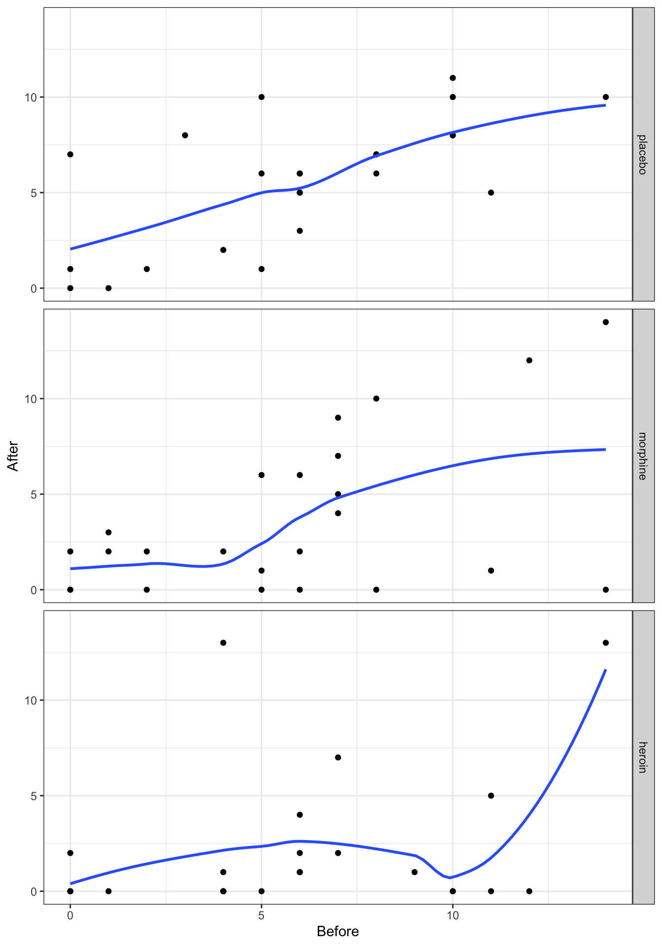
圖 58.1: Lowess smoother, with bandwith/span set to 0.8, for the mental data
ggplot(Mental, aes(Before, After)) + geom_point() +
  geom_smooth(method = "loess",  span = 0.4, se = FALSE) +
  facet_grid(treatment ~ .) + theme_bw()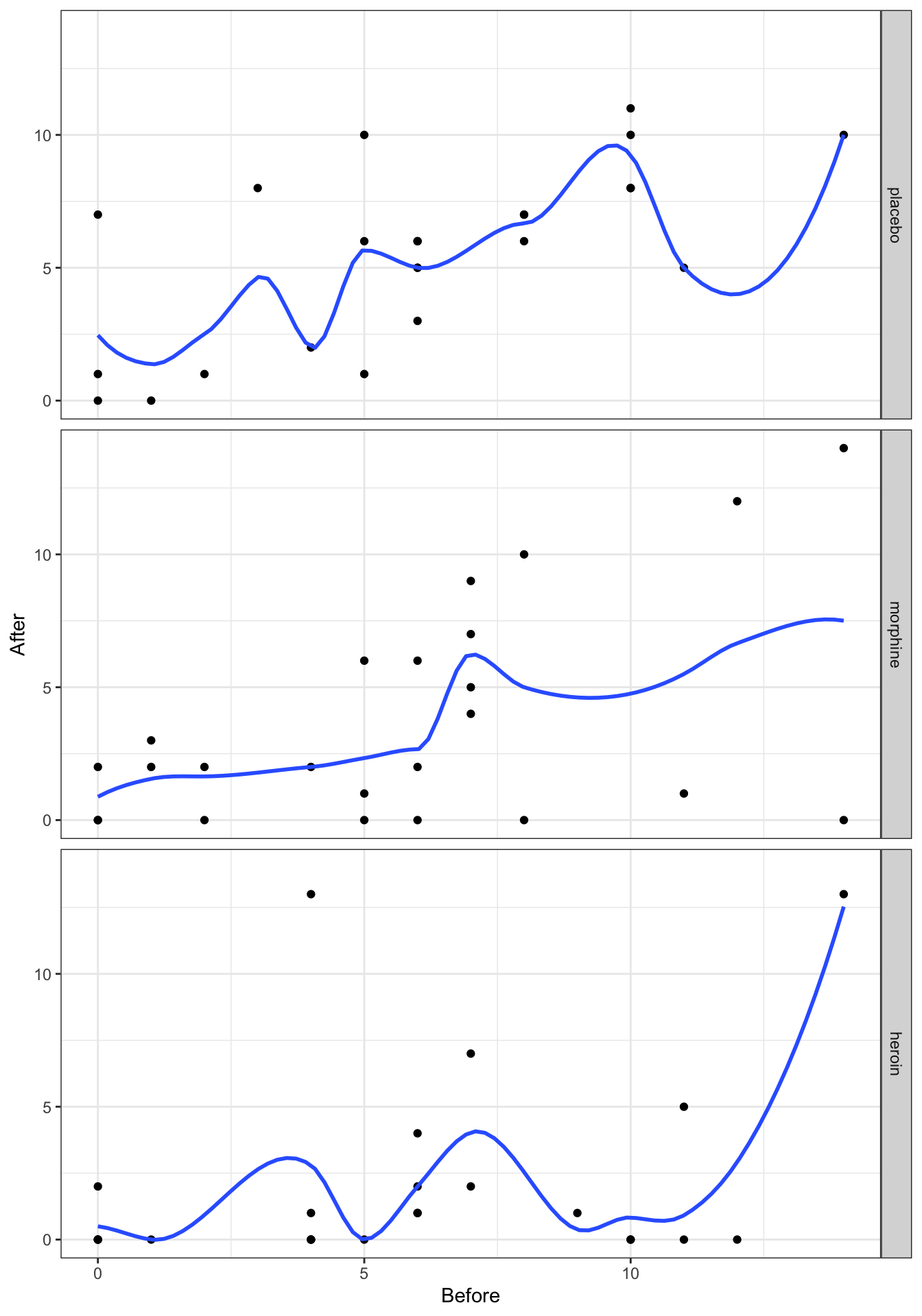
圖 58.2: Lowess smoother, with bandwith/span set to 0.4, for the mental data
58.5 GLM-Practical 02
58.5.1 思考本章中指數分布家族的參數設置。假如,有一個觀測值 \(y\) 來自指數家族。試求證:
MLE \(\hat\theta\) 是 \(b^\prime(\theta) = y\) 的解;
\(\theta\) 的 MLE 的方差是 \(\frac{\phi}{b^{\prime\prime}(\theta)}\);
如果 \(Y\sim N(\mu, \sigma^2)\),試進一步證明 \(b^\prime(\theta) = \mu\) 且 \(\frac{\phi}{b^{\prime\prime}(\theta)} = \sigma^2\)
當數據來自指數分布家族,它的對數似然可以寫作:
\[ \frac{y\cdot\theta - b(\theta)}{\phi} - c(y, \phi) \]
對這個對數似然方程取 \(\theta\) 的偏微分方程可得:
\[ \frac{\partial}{\partial\theta}\ell(\theta,\phi) = \frac{y - b^\prime(\theta)}{\phi} \]
令此偏微分方程等於零,那麼我們可以知道 \(\hat\theta\) 是 \(b^\prime(\theta) = y\) 的解。
- MLE 的方差可以用 Fisher information 來推導。
\[ S^2=\left.-\frac{1}{\ell^{\prime\prime}(\theta)}\right\vert_{\theta=\hat{\theta}} \\ \text{Because } \ell^{\prime\prime}(\theta) = -\frac{b^{\prime\prime}(\theta)}{\phi} \\ \Rightarrow S^2 = \frac{\phi}{b^{\prime\prime}(\theta)} \]
- 如果 \(Y\sim N(\mu, \sigma^2)\), 那麼,根據正態分布數據屬於指數家族的性質,
\[ \phi = \sigma^2,\theta = \mu, b(\theta =\mu) = \frac{\mu^2}{2} \\ \Rightarrow b^\prime(\theta) = \mu \\ \Rightarrow S^2 = \frac{\phi}{b^{\prime\prime}(\theta)} = \sigma^2 \]
58.5.2 R 練習
數據來自一個RCT臨牀試驗,比較嗎啡,海洛因和安慰劑在患者精神狀態評分上的影響,試分析數據回答下面的問題:
- 三組治療組之間注射後的評分均值不同嗎?
- 調整基線時精神狀態評分對你的模型結果有什麼影響?
- 基線時精神狀態評分的高低會影響不同藥物的效果嗎?
58.5.2.1 數據讀入 R,作初步分析
Mental <- read.table("../backupfiles/MENTAL.DAT", header =  FALSE, sep ="", col.names = c("treatment", "prement", "mentact"))
Mental$treatment[Mental$treatment == 1] <- "placebo"
Mental$treatment[Mental$treatment == 2] <- "morphine"
Mental$treatment[Mental$treatment == 3] <- "heroin"
Mental$treatment <- factor(Mental$treatment, levels = c("placebo", "morphine", "heroin"))
head(Mental)
## treatment prement mentact
## 1 placebo 0 7
## 2 placebo 2 1
## 3 placebo 14 10
## 4 placebo 5 10
## 5 placebo 5 6
## 6 placebo 4 2# Use hsitograms and plots to look at the distributions of the pre- and post- injection scores.
# with(Mental, hist(prement, breaks = 14, freq = F))
# qplot(prement, data = Mental, binwidth = 1)
hist1 <- ggplot(Mental, aes(x = prement, y = ..density..)) + geom_histogram(binwidth = 1) + theme_bw()
hist2 <- ggplot(Mental, aes(x = mentact, y = ..density..)) + geom_histogram(binwidth = 1) + theme_bw()
Scatter <- ggplot(Mental, aes(x = prement, y = mentact)) + geom_point()+ theme_bw()
grid.arrange(hist1, hist2, Scatter, ncol=2)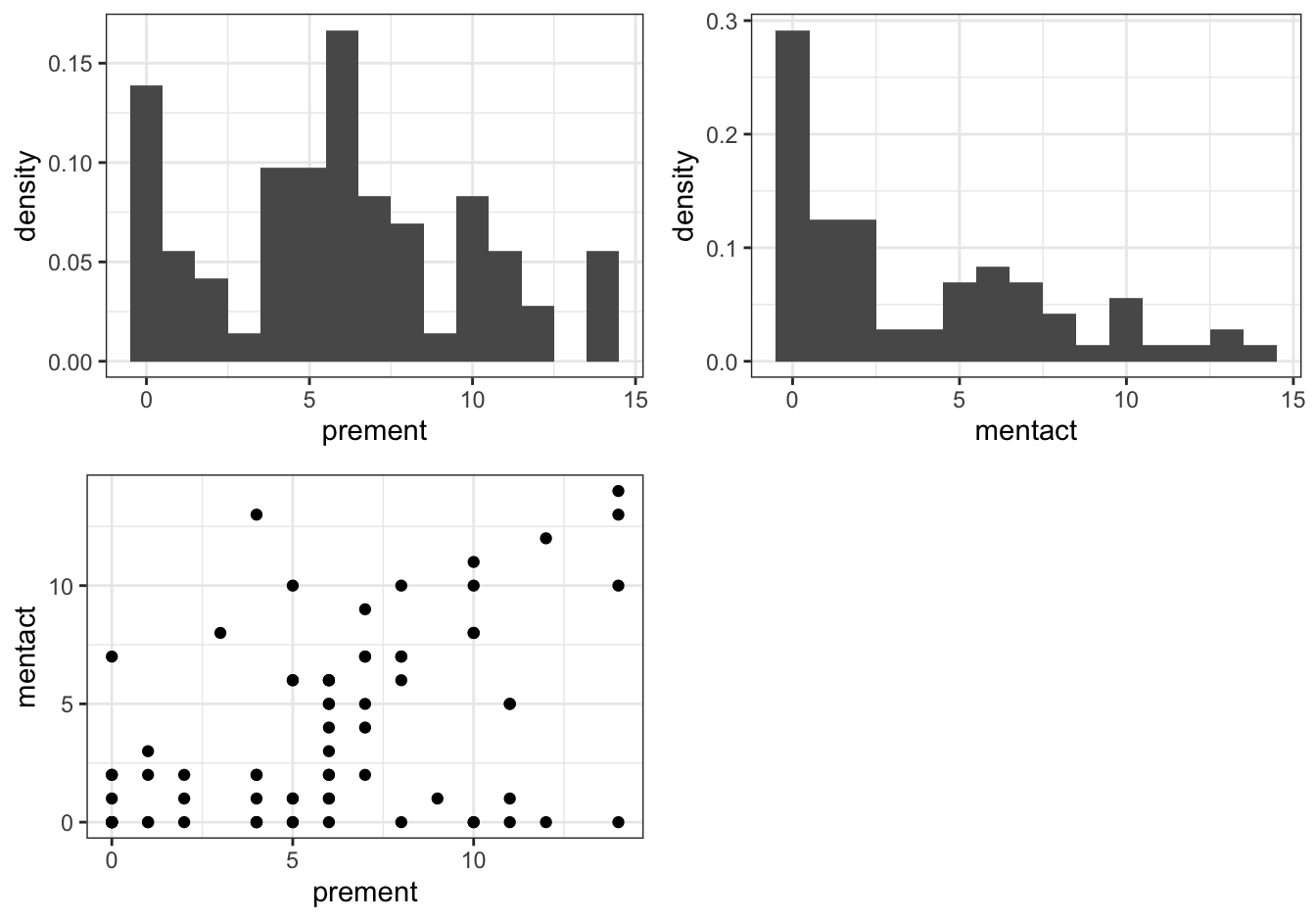
圖 58.3: Histogram and plots
可以看到柱狀圖暗示我們實驗前後的得分本身都不服從正態分布。但是這並不妨礙我們使用回歸模型來做推斷。畢竟,線性回歸模型只要求殘差服從正態分布。另外,散點圖提示實驗前後的得分之間可能呈正相關。
ggplot(Mental, aes(prement, mentact)) + geom_point() +
  geom_smooth(method = "loess",  span = 0.8, se = FALSE) +
  facet_grid(treatment ~ .) + theme_bw()
## `geom_smooth()` using formula 'y ~ x'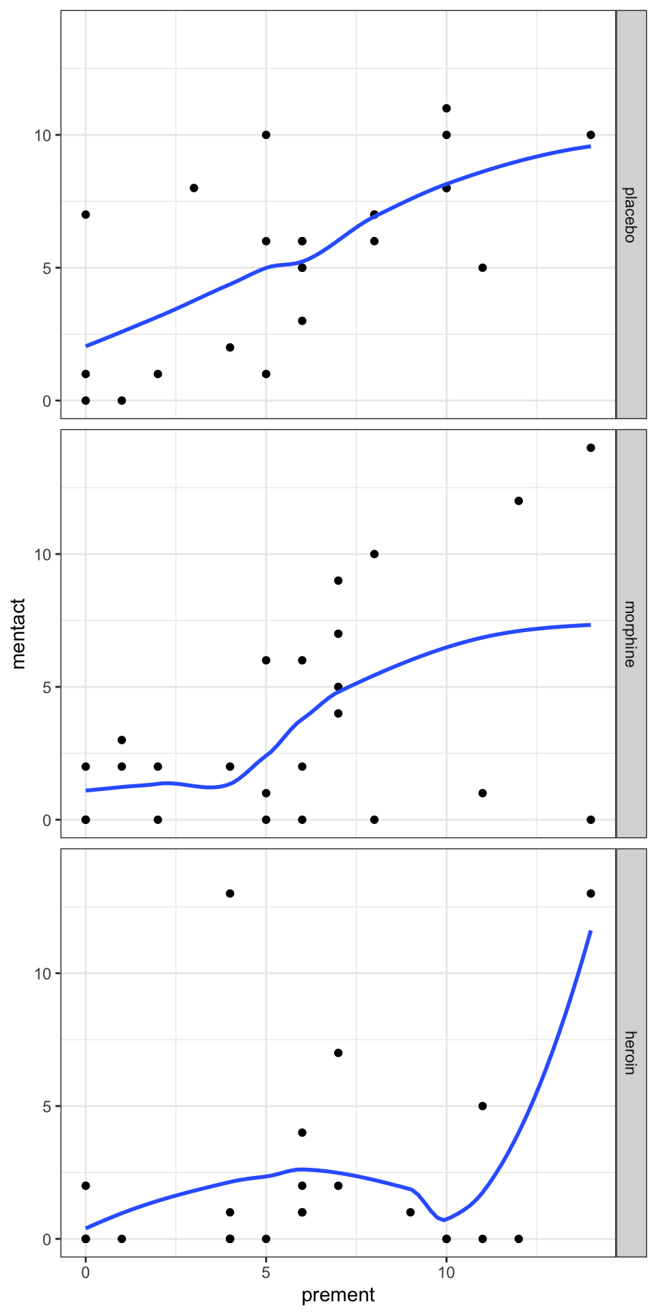
圖 58.4: Lowess smoother, with bandwith/span set to 0.8, for the mental data
對於每組實驗組來說,觀測值數量都很少,姑且可以認爲線性模型是合理的。
| Terms fitted | RSS | Residuals df |
|---|---|---|
|
1117.875 | 71 |
|
980.625 | 69 |
|
884.328 | 70 |
|
752.055 | 68 |
|
733.127 | 66 |
58.5.2.2 寫下表格 58.1 中五個線性回歸模型的數學表達式,在 R 裏面擬合這5個模型,在第二列第三列分別填寫各模型的統計信息 (殘差平方和 residuals sum of squares,和 殘差自由度 reiduals degrees of freedom)。利用該表格填寫完整以後的內容,用筆和紙正式地比較模型 3 和 4; 4 和 5 的擬合優度。然後和 R 的輸出結果比較確認。你會作出怎樣的結論?另外,爲什麼相似的比較模型的方法不適用於比較模型 2 和 3?
解
用 \(z_i, y_i\) 分別標記第 \(i\) 名患者在藥物注射前,後兩次測量的精神醫學指徵評分。使用線性回歸模型的前提假設是 \(y_i \sim N(\mu_i, \sigma^2)\) 且互相獨立。另外,預測變量的標記爲:
\[ x_{1i} = \left\{ \begin{array}{ll} 0 \text{ placebo or heroin }\\ 1 \text{ morphine}\\ \end{array} \right. x_{2i} = \left\{ \begin{array}{ll} 0 \text{ placebo or morphine }\\ 1 \text{ heroin}\\ \end{array} \right. \\ \]
- Overall mean model
鏈接方程部分: \(\eta_i = \beta_0\)
##
## Call:
## lm(formula = mentact ~ 1, data = Mental)
##
## Residuals:
##     Min      1Q  Median      3Q     Max
## -3.7917 -3.7917 -1.7917  2.4583 10.2083
##
## Coefficients:
##             Estimate Std. Error t value  Pr(>|t|)
## (Intercept)  3.79167    0.46763  8.1083 1.053e-11 ***
## ---
## Signif. codes:  0 '***' 0.001 '**' 0.01 '*' 0.05 '.' 0.1 ' ' 1
##
## Residual standard error: 3.968 on 71 degrees of freedom## Analysis of Variance Table
##
## Response: mentact
## Df Sum Sq Mean Sq F value Pr(>F)
## Residuals 71 1117.88 15.7447- Drugs model
鏈接方程部分: \(\eta_i = \beta_0 + \beta_1 x_{1i} + \beta_2 x_{2i}\)
##
## Call:
## lm(formula = mentact ~ treatment, data = Mental)
##
## Residuals:
##     Min      1Q  Median      3Q     Max
## -5.5417 -2.1667 -1.1667  1.9583 10.8333
##
## Coefficients:
##                   Estimate Std. Error t value  Pr(>|t|)
## (Intercept)        5.54167    0.76952  7.2014 5.732e-10 ***
## treatmentmorphine -1.87500    1.08827 -1.7229  0.089382 .
## treatmentheroin   -3.37500    1.08827 -3.1013  0.002791 **
## ---
## Signif. codes:  0 '***' 0.001 '**' 0.01 '*' 0.05 '.' 0.1 ' ' 1
##
## Residual standard error: 3.7699 on 69 degrees of freedom
## Multiple R-squared:  0.12278,    Adjusted R-squared:  0.097351
## F-statistic: 4.8287 on 2 and 69 DF, p-value: 0.010896## Analysis of Variance Table
##
## Response: mentact
## Df Sum Sq Mean Sq F value Pr(>F)
## treatment 2 137.250 68.625 4.82868 0.010896 *
## Residuals 69 980.625 14.212
## ---
## Signif. codes: 0 '***' 0.001 '**' 0.01 '*' 0.05 '.' 0.1 ' ' 1- Pre-inj model
鏈接方程部分 \(\eta_i = \beta_0 + \beta_3 z_i\)
##
## Call:
## lm(formula = mentact ~ prement, data = Mental)
##
## Residuals:
##      Min       1Q   Median       3Q      Max
## -7.51879 -2.32837 -0.89028  2.25419 10.06844
##
## Coefficients:
##             Estimate Std. Error t value   Pr(>|t|)
## (Intercept)  1.09667    0.75388  1.4547     0.1502
## prement      0.45872    0.10669  4.2996 0.00005433 ***
## ---
## Signif. codes:  0 '***' 0.001 '**' 0.01 '*' 0.05 '.' 0.1 ' ' 1
##
## Residual standard error: 3.5543 on 70 degrees of freedom
## Multiple R-squared:  0.20892,    Adjusted R-squared:  0.19762
## F-statistic: 18.487 on 1 and 70 DF, p-value: 0.000054335## Analysis of Variance Table
##
## Response: mentact
## Df Sum Sq Mean Sq F value Pr(>F)
## prement 1 233.547 233.5473 18.4867 0.000054335 ***
## Residuals 70 884.328 12.6333
## ---
## Signif. codes: 0 '***' 0.001 '**' 0.01 '*' 0.05 '.' 0.1 ' ' 1- Drugs + pre-inj model
鏈接方程部分: \(\eta_i = \beta_0 + \beta_1 x_{1i} + \beta_2 x_{2i} + \beta_3z_i\)
#4.  Drugs + Pre-inj model
Drug_Pre_inj <- lm(mentact ~ treatment + prement, data = Mental)
summary(Drug_Pre_inj)
##
## Call:
## lm(formula = mentact ~ treatment + prement, data = Mental)
##
## Residuals:
## Min 1Q Median 3Q Max
## -7.41185 -2.05478 -0.22877 1.08012 11.68451
##
## Coefficients:
## Estimate Std. Error t value Pr(>|t|)
## (Intercept) 2.817898 0.905424 3.1122 0.0027149 **
## treatmentmorphine -1.761510 0.960344 -1.8342 0.0709923 .
## treatmentheroin -3.318255 0.960100 -3.4562 0.0009488 ***
## prement 0.453961 0.099857 4.5461 0.00002308 ***
## ---
## Signif. codes: 0 '***' 0.001 '**' 0.01 '*' 0.05 '.' 0.1 ' ' 1
##
## Residual standard error: 3.3256 on 68 degrees of freedom
## Multiple R-squared: 0.32725, Adjusted R-squared: 0.29757
## F-statistic: 11.026 on 3 and 68 DF, p-value: 5.4921e-06## Analysis of Variance Table
##
## Response: mentact
## Df Sum Sq Mean Sq F value Pr(>F)
## treatment 2 137.250 68.6250 6.20499 0.0033478 **
## prement 1 228.570 228.5696 20.66700 0.00002308 ***
## Residuals 68 752.055 11.0596
## ---
## Signif. codes: 0 '***' 0.001 '**' 0.01 '*' 0.05 '.' 0.1 ' ' 1- Drug + Pre-inj + Drug×Pre-inj
鏈接方程部分: \(\eta_i = \beta_0 + \beta_1 x_{1i} + \beta_2 x_{2i} + \beta_3 z_i + \beta_{13}x_{1i}z_i + \beta_{23}x_{2i}z_i\)
#5.  Drugs + Pre-inj + Drug×Pre-inj model
Model5 <- lm(mentact ~ treatment*prement, data = Mental)
summary(Model5)
##
## Call:
## lm(formula = mentact ~ treatment * prement, data = Mental)
##
## Residuals:
## Min 1Q Median 3Q Max
## -7.82808 -1.93513 -0.51606 1.41607 11.36012
##
## Coefficients:
## Estimate Std. Error t value Pr(>|t|)
## (Intercept) 1.978030 1.294069 1.5285 0.131158
## treatmentmorphine -1.211742 1.750342 -0.6923 0.491185
## treatmentheroin -1.461968 1.771855 -0.8251 0.412284
## prement 0.593939 0.183468 3.2373 0.001889 **
## treatmentmorphine:prement -0.089526 0.248346 -0.3605 0.719633
## treatmentheroin:prement -0.312985 0.250383 -1.2500 0.215704
## ---
## Signif. codes: 0 '***' 0.001 '**' 0.01 '*' 0.05 '.' 0.1 ' ' 1
##
## Residual standard error: 3.3329 on 66 degrees of freedom
## Multiple R-squared: 0.34418, Adjusted R-squared: 0.29449
## F-statistic: 6.9274 on 5 and 66 DF, p-value: 0.000029744## Analysis of Variance Table
##
## Response: mentact
## Df Sum Sq Mean Sq F value Pr(>F)
## treatment 2 137.250 68.6250 6.17798 0.0034719 **
## prement 1 228.570 228.5696 20.57704 0.000024811 ***
## treatment:prement 2 18.928 9.4639 0.85199 0.4312025
## Residuals 66 733.128 11.1080
## ---
## Signif. codes: 0 '***' 0.001 '**' 0.01 '*' 0.05 '.' 0.1 ' ' 1比較模型 3 和 4 可以使用相關的 F 統計量 (Partial F tests)
\[ F=\frac{(844.328 - 752.055)/(70-68)}{752.055/68} = 5.98 \]
自由度爲 (2,68) 時 F 統計量爲 5.98 的概率是:
## [1] 0.0040516165所以我們有極強的證據證明這兩個模型顯著不同,且模型 4 擬合數據更好,且該證據也證明了注射藥物後三組之間的精神醫學指徵的分顯著不同。用 R 進行偏 F 檢驗如下,可見我們的計算是完全正確的:
## Analysis of Variance Table
##
## Model 1: mentact ~ prement
## Model 2: mentact ~ treatment + prement
##   Res.Df     RSS Df Sum of Sq       F    Pr(>F)
## 1     70 884.328
## 2     68 752.055  2   132.272 5.97996 0.0040518 **
## ---
## Signif. codes:  0 '***' 0.001 '**' 0.01 '*' 0.05 '.' 0.1 ' ' 1
比較模型 4 和 5:
## Analysis of Variance Table
##
## Model 1: mentact ~ treatment + prement
## Model 2: mentact ~ treatment * prement
##   Res.Df     RSS Df Sum of Sq       F Pr(>F)
## 1     68 752.055
## 2     66 733.128  2   18.9278 0.85199 0.4312
所以,模型 4 和 5 比較的結果告訴我們沒有證據證明實驗前的精神醫學指徵得分和不同治療組之間有交互作用。但是由於模型 2 和 3 本身不是互爲嵌套式結構的,所以他們無法通過相似的偏 F 檢驗來比較模型。
58.5.2.3 用 glm 命令擬合模型 4,試比較其輸出結果和 lm 之間的異同:
Model4 <- glm(mentact ~ treatment + prement, family = gaussian(link = "identity"), data = Mental)
summary(Model4)
##
## Call:
## glm(formula = mentact ~ treatment + prement, family = gaussian(link = "identity"),
## data = Mental)
##
## Deviance Residuals:
## Min 1Q Median 3Q Max
## -7.41185 -2.05478 -0.22877 1.08012 11.68451
##
## Coefficients:
## Estimate Std. Error t value Pr(>|t|)
## (Intercept) 2.817898 0.905424 3.1122 0.0027149 **
## treatmentmorphine -1.761510 0.960344 -1.8342 0.0709923 .
## treatmentheroin -3.318255 0.960100 -3.4562 0.0009488 ***
## prement 0.453961 0.099857 4.5461 0.00002308 ***
## ---
## Signif. codes: 0 '***' 0.001 '**' 0.01 '*' 0.05 '.' 0.1 ' ' 1
##
## (Dispersion parameter for gaussian family taken to be 11.059638)
##
## Null deviance: 1117.875 on 71 degrees of freedom
## Residual deviance: 752.055 on 68 degrees of freedom
## AIC: 383.25
##
## Number of Fisher Scoring iterations: 2可以看出各個參數估計和標準誤估計都是完全相同的。但是當你使用 STATA 的 glm 命令時,它默認的高斯鏈接方程使用的不是 t 檢驗結果而是 z 檢驗結果,所以會給出略微不同的 95% 信賴區間。
58.5.2.4 使用相關模型的結果填寫下列表格
| Mean | Mean diff with Placebo | SE | Adj. mean diff with Placebo | SE | |
|---|---|---|---|---|---|
| Placebo | 5.542 | 0.000 | – | 0.000 | – |
| Morphine | 3.667 | -1.875 | 1.08 | -1.761 | 0.96 |
| Heroin | 2.167 | -3.375 | 1.08 | -3.310 | 0.96 |
58.5.2.5 對分析的結果做簡短的總結
在模型 2 (drug model) 中,F 檢驗給出的 p = 0.0109,提供了較爲有力的證據證明每個治療組治療後的精神醫學指徵得分是不同的。但是,觀察每個回歸系數的檢驗結果,發現嗎啡組和安慰劑組之差其實沒有達到 5% 統計學意義 (p = 0.089),海洛因組和安慰劑組之間的得分差則達到了 5% 的統計學意義 (p = 0.003)。
模型加入對實驗前精神醫學指徵得分的調整之後,組與組之間的估計差發生了些許(但是並不大)的變化。這其實也是我們事先估計的結果,因爲對於RCT來說,沒有混雜因素,之所以調整基線值,主要爲的是提升參數估計的精確度 (減小 SE,從而使95% 信賴區間更小)。
對交互作用實施了偏 F 檢驗得到的結果 (p = 0.43) 提示,沒有證據反對零假設 – 藥物作用效果不因爲實驗前患者的精神醫學指徵得分不同而不同。
最後,glm 和 lm 的模型結果輸出在 R 裏是幾乎完全相同的,在 STATA 裏面則有計算方法的不同導致不同的95%CI。