第 62 章率的廣義線性迴歸 Poisson GLM for rates

62.1 醫學中的率

前章介紹的事件發生次數，使用的是泊松迴歸。本章介紹同樣利用泊松迴歸，對事件發生率類型數據的泊松迴歸模型。常見的率的數據例如：

肺癌發病率
工廠職工的死亡率
術後後遺症的發生率

下列數據來自英國醫生調查 (British doctors study)，研究的是男性醫生中吸菸與否和冠心病死亡之間的關係。最後一列是每組觀測對象被追蹤的人年 (person-year)。

##    agegrp     smokes deaths  pyrs
## 1   35-44     Smoker     32 52407
## 2   45-54     Smoker    104 43248
## 3   55-64     Smoker    206 28612
## 4   65-74     Smoker    186 12663
## 5     75+     Smoker    102  5317
## 6   35-44 Non-smoker      2 18790
## 7   45-54 Non-smoker     12 10673
## 8   55-64 Non-smoker     28  5710
## 9   65-74 Non-smoker     28  2585
## 10    75+ Non-smoker     31  1462

這是一個已經被整理過的數據，我們沒有辦法從這樣的數據還原到每個觀察對象的個人水平數據。冠心病的粗死亡率 (crude death rate) 可以被計算如下表 (忽略年齡分組)，此時默認的前提是死亡事件在追蹤的過程中發生的概率不發生改變。

表 62.1: Death rates due to CHD in smokers and non-smokers, collapsed over age group
Group	Person-years of follow-up	CHD deaths	Death Rate per 1000 person-years	Rate Ratios
Non-smokers	39220	101	2.58	1.00
Smokers	142247	630	4.43	1.72

62.2 泊松過程

設 \(Y\) 是代表某段時間 \(t\) 內事件發生次數 (死亡) 的隨機變量。如果可以假設：

每次事件的發生，是互相獨立的，即在沒有重疊的時間線上，每個事件的發生是隨機的。
在一個無限小的時間段 \(\delta t\) 內，事件發生的概率是 \(\lambda\times\delta t\)，其中 \(\delta t \rightarrow 0\)。

那麼根據泊松分佈 (Section 6) 的定義，在這個時間段內，隨機變量 \(Y\) 事件發生次數服從泊松分佈：

\[ \begin{aligned} Y & \sim \text{Po}(\mu) \\ \text{Where } \mu & = \lambda t, \text{ and } \lambda \text{ is the Rate} \end{aligned} \]

所以，從泊松過程可以看到，我們關心的參數是事件發生率 \(\lambda\)。

62.3 率的模型

既然關心的參數只是發生率，且我們已知泊松分佈是指數分佈的家族成員，可以用廣義線性模型的概念來建模。

因變量分佈，distribution of dependent variable \[Y_i \sim \text{Po}(\mu_i), \text{ where } \mu_i = \lambda_i t_i\]
線性預測方程，linear predictor \[\eta_i = \alpha + \beta_1 x_{i1} + \cdots + \beta_p x_{ip}\]
標準鏈接方程，canonical link function \[\text{log}(\lambda_i) = \text{log}(\frac{\mu_i}{t_i})\]

所以，將率的模型整理一下，就變成了

\[ \begin{aligned} \text{log}(\mu_i) - \text{log}(t_i) & = \alpha + \beta_1 x_{i1} + \cdots + \beta_p x_{ip} \\ \text{log}(\mu_i) & = \text{log}(t_i) + \alpha + \beta_1 x_{i1} + \cdots + \beta_p x_{ip} \end{aligned} \]

你可以看到，時間項的對數部分 \(\text{log}(t_i)\) 其實是被移到線性預測方程的右邊跟參數放在一起的，只是它的迴歸係數被強制爲 \(1\)。這個時間項被叫做 補償項 (offset)。這樣我們就成功地擬合了用於求事件發生率的一個泊松迴歸模型。在 R 裏，你可以用 glm() 命令的 offset = 選項功能，也可以把 offset(log(Person-year)) 作爲線性預測方程的一部分把時間項取對數以後放進模型裏面。

62.4 率的 GLM

所以我們一起來把率的 GLM 正式定義一下，它包含三個部分：

可被認爲互相獨立的因變量觀測值的分佈服從泊松分佈 \[Y_i \sim \text{Po}(\mu_i)\]
其中 \(E(Y_i) = \mu_i = \lambda_i t_i\)，\(t_i\) 是第 \(i\) 個觀察對象 (或者觀察組) 的追蹤人年 (person-time)。
線性預測方程 \[\eta_i = \text{log}(t_i) + \alpha + \beta_1 x_{i1} + \cdots + \beta_p x_{ip}\]
鏈接方程是均值的對數方程 \[\text{log}(\mu_i) = \eta_i\]

和分組型二項分佈數據相似，如果泊松 GLM 擬合的數據也是分組型數據，如本章開頭的英國醫生隊列數據。那麼模型偏差值 (deviance) 可以用來衡量模型擬合的好壞。在零假設條件下，模型偏差值服從自由度爲 \(n-p\) 的卡方分佈 (這裏的 \(n\) 是分組型數據中的“組的數量”，也就是飽和模型中參數的數量，\(p\) 是擬合的線性預測方程中參數的數量)。

62.5 分析實例 Example: British doctors study

數據是本章開頭使用的英國醫生隊列

##    agegrp     smokes deaths  pyrs
## 1   35-44     Smoker     32 52407
## 2   45-54     Smoker    104 43248
## 3   55-64     Smoker    206 28612
## 4   65-74     Smoker    186 12663
## 5     75+     Smoker    102  5317
## 6   35-44 Non-smoker      2 18790
## 7   45-54 Non-smoker     12 10673
## 8   55-64 Non-smoker     28  5710
## 9   65-74 Non-smoker     28  2585
## 10    75+ Non-smoker     31  1462

每組的死亡人數用 \(y_i, i=1,\cdots,10\) 標記；
每組追蹤的人年用 \(t_i\) 標記；
\(x_{i1} = 0\) 時對象是吸菸者，\(x_{i1} = 1\) 時對象是非吸菸者；
\(x_{i2}, x_{i3}, x_{i4}, x_{i5}\) 作爲5個年齡組的啞變量。

分析目的是：

調查吸菸與冠心病死亡率的關係 (不調整年齡)；
調查吸菸與冠心病死亡率的年齡調整後關係；
調查年齡是否對吸菸與冠心病死亡率的關係起到交互作用。

62.5.1 模型 1: 吸菸

第一個模型可以用下面的數學表達式：

\[ \text{log}(\mu_i) = \text{log}(t_i) + \alpha + \beta_1 x_{i1} \]

在 R 裏面用下面的代碼來擬合這個模型，仔細閱讀輸出的結果：

# the following 2 models are equivalent
Model1 <- glm(deaths ~ smokes + offset(log(pyrs)), family = poisson(link = "log"), data = BritishD)
Model1 <- glm(deaths ~ smokes, offset = log(pyrs), family = poisson(link = "log"), data = BritishD)
summary(Model1); jtools::summ(Model1, digits = 6, confint = TRUE, exp = TRUE)

## 
## Call:
## glm(formula = deaths ~ smokes, family = poisson(link = "log"), 
##     data = BritishD, offset = log(pyrs))
## 
## Deviance Residuals: 
##      Min        1Q    Median        3Q       Max  
## -16.5348   -6.0313    4.6116    8.1617   13.6441  
## 
## Coefficients:
##               Estimate Std. Error  z value  Pr(>|z|)    
## (Intercept)  -5.961822   0.099504 -59.9157 < 2.2e-16 ***
## smokesSmoker  0.542221   0.107183   5.0588 4.219e-07 ***
## ---
## Signif. codes:  0 '***' 0.001 '**' 0.01 '*' 0.05 '.' 0.1 ' ' 1
## 
## (Dispersion parameter for poisson family taken to be 1)
## 
##     Null deviance: 935.067  on 9  degrees of freedom
## Residual deviance: 905.976  on 8  degrees of freedom
## AIC: 965.044
## 
## Number of Fisher Scoring iterations: 6

Observations	10
Dependent variable	deaths
Type	Generalized linear model
Family	poisson
Link	log

𝛘²(1)	29.091145
Pseudo-R² (Cragg-Uhler)	0.945476
Pseudo-R² (McFadden)	0.029381
AIC	965.044126
BIC	965.649296

	exp(Est.)	2.5%	97.5%	z val.	p
(Intercept)	0.002575	0.002119	0.003130	-59.915661	0.000000
smokesSmoker	1.719823	1.393956	2.121867	5.058821	0.000000
Standard errors: MLE

輸出報告中的參數估計部分 Estimate 就是我們擬合模型中參數的估計 \(\hat\alpha, \hat\beta_1\)，他們各自的含義是：

\(\hat\alpha = -5.96\)：非吸菸者的冠心病估計死亡率的對數 (the estimated log rate for non-smokers)；
\(\hat\beta_1 = 0.547\)：非吸菸者和吸菸者兩組之間冠心病死亡率對數之差 (the estimated difference in log rate between non-smokers and smokers)。

注意看報告中間部分模型偏差部分的數字 Residual deviance: 905.98 on 8 degrees of freedom，如果對模型 1 進行擬合優度檢驗：

with(Model1, cbind(res.deviance = deviance, df = df.residual,
  p = pchisq(deviance, df.residual, lower.tail=FALSE)))

##      res.deviance df              p
## [1,]    905.97619  8 2.9024145e-190

擬合優度檢驗結果提示，這個模型對數據的擬合非常差 (poor fit)。可能的原因是，模型 1 中忽略了“年齡”這一重要的因素，使得當僅僅使用吸菸與否的信息擬合的泊松迴歸模型的擬合值和觀察值之間的差異的波動非常大，大到很可能無法滿足泊松分佈的前提假設。

62.5.2 模型 2: 吸菸 + 年齡

第二個模型的線性預測方程可以寫作：

\[ \text{log}(\mu_i) = \text{ln}(t_i) + \alpha + \beta_1 x_{i1} + \beta_2 x_{i2} + \beta_3 x_{i3} + \beta_4 x_{i4} + \beta_5 x_{i5} \]

在 R 裏面用下面的代碼來擬合這個模型，仔細閱讀輸出的結果：

Model2 <- glm(deaths ~ smokes + agegrp + offset(log(pyrs)), family = poisson(link = "log"), data = BritishD)
summary(Model2); jtools::summ(Model2, digits = 6, confint = TRUE, exp = TRUE)

## 
## Call:
## glm(formula = deaths ~ smokes + agegrp + offset(log(pyrs)), family = poisson(link = "log"), 
##     data = BritishD)
## 
## Deviance Residuals: 
##         1          2          3          4          5          6          7          8          9  
##  0.901600   0.510379   0.051347  -0.087318  -0.912369  -2.179780  -1.308000  -0.137907   0.228819  
##        10  
##  1.919020  
## 
## Coefficients:
##              Estimate Std. Error  z value  Pr(>|z|)    
## (Intercept)  -7.91933    0.19176 -41.2978 < 2.2e-16 ***
## smokesSmoker  0.35454    0.10737   3.3019 0.0009604 ***
## agegrp45-54   1.48401    0.19510   7.6063 2.821e-14 ***
## agegrp55-64   2.62751    0.18373  14.3012 < 2.2e-16 ***
## agegrp65-74   3.35049    0.18480  18.1305 < 2.2e-16 ***
## agegrp75+     3.70010    0.19222  19.2494 < 2.2e-16 ***
## ---
## Signif. codes:  0 '***' 0.001 '**' 0.01 '*' 0.05 '.' 0.1 ' ' 1
## 
## (Dispersion parameter for poisson family taken to be 1)
## 
##     Null deviance: 935.0673  on 9  degrees of freedom
## Residual deviance:  12.1324  on 4  degrees of freedom
## AIC: 79.2003
## 
## Number of Fisher Scoring iterations: 4

Observations	10
Dependent variable	deaths
Type	Generalized linear model
Family	poisson
Link	log

𝛘²(5)	922.934964
Pseudo-R² (Cragg-Uhler)	1.000000
Pseudo-R² (McFadden)	0.932130
AIC	79.200307
BIC	81.015817

	exp(Est.)	2.5%	97.5%	z val.	p
(Intercept)	0.000364	0.000250	0.000530	-41.297843	0.000000
smokesSmoker	1.425519	1.154984	1.759421	3.301875	0.000960
agegrp45-54	4.410584	3.009014	6.464990	7.606281	0.000000
agegrp55-64	13.839200	9.654338	19.838070	14.301161	0.000000
agegrp65-74	28.516783	19.851789	40.963909	18.130508	0.000000
agegrp75+	40.451206	27.753285	58.958789	19.249382	0.000000
Standard errors: MLE

此時可以計算吸菸者與非吸菸者相比時，年齡調整後冠心病死亡率的比爲：

\[ \begin{aligned} e^{0.3545} & = 1.43 \text{ with } 95\% \text{ CI: } \\ (e^{0.3545 - 1.96\times0.1074}, & e^{0.3545 + 1.96\times0.1074}) = (1.16, 1.76) \end{aligned} \]

報告中還包含了對吸菸項迴歸係數的 Wald 檢驗結果 smokesSmoker 0.3545 0.1074 3.302 0.00096 ***，從這一結果來看，數據提供了強有力的證據證明了年齡調整以後，吸菸會引起冠心病死亡率的顯著升高。再利用模型擬合報告中模型偏差部分的數據 Residual deviance: 905.98 on 8 degrees of freedom，模型的擬合優度檢驗結果爲：

with(Model2, cbind(res.deviance = deviance, df = df.residual,
  p = pchisq(deviance, df.residual, lower.tail=FALSE)))

##      res.deviance df           p
## [1,]    12.132366  4 0.016393625

結果依然提示，即使把年齡組放入這個泊松迴歸，模型對數據的擬合程度依然非常的不好。所以，到這裏，在即使調整了年齡之後模型擬合度依然不理想的情況下 (這是需要加交互作用項的證據)，我們需要在模型中加入年齡和吸菸的交互作用項 (結果是加入交互作用項的模型就變成了飽和模型)。

62.5.3 模型 3: 吸菸 + 年齡 + 吸菸與年齡的交互作用項

Model3 <- glm(deaths ~ smokes*agegrp + offset(log(pyrs)), 
              family = poisson(link = "log"), data = BritishD)
summary(Model3); jtools::summ(Model3, digits = 6, confint = TRUE, exp = TRUE)

## 
## Call:
## glm(formula = deaths ~ smokes * agegrp + offset(log(pyrs)), family = poisson(link = "log"), 
##     data = BritishD)
## 
## Deviance Residuals: 
##  [1]  0  0  0  0  0  0  0  0  0  0
## 
## Coefficients:
##                          Estimate Std. Error  z value  Pr(>|z|)    
## (Intercept)              -9.14793    0.70711 -12.9371 < 2.2e-16 ***
## smokesSmoker              1.74687    0.72887   2.3967  0.016544 *  
## agegrp45-54               2.35737    0.76376   3.0865  0.002025 ** 
## agegrp55-64               3.83016    0.73192   5.2330 1.668e-07 ***
## agegrp65-74               4.62266    0.73192   6.3158 2.688e-10 ***
## agegrp75+                 5.29436    0.72956   7.2569 3.960e-13 ***
## smokesSmoker:agegrp45-54 -0.98662    0.79006  -1.2488  0.211741    
## smokesSmoker:agegrp55-64 -1.36281    0.75619  -1.8022  0.071512 .  
## smokesSmoker:agegrp65-74 -1.44229    0.75653  -1.9065  0.056592 .  
## smokesSmoker:agegrp75+   -1.84699    0.75717  -2.4393  0.014715 *  
## ---
## Signif. codes:  0 '***' 0.001 '**' 0.01 '*' 0.05 '.' 0.1 ' ' 1
## 
## (Dispersion parameter for poisson family taken to be 1)
## 
##     Null deviance:  9.35067e+02  on 9  degrees of freedom
## Residual deviance: -2.30926e-14  on 0  degrees of freedom
## AIC: 75.0679
## 
## Number of Fisher Scoring iterations: 3

Observations	10
Dependent variable	deaths
Type	Generalized linear model
Family	poisson
Link	log

𝛘²(9)	935.067331
Pseudo-R² (Cragg-Uhler)	1.000000
Pseudo-R² (McFadden)	0.944383
AIC	75.067940
BIC	78.093791

	exp(Est.)	2.5%	97.5%	z val.	p
(Intercept)	0.000106	0.000027	0.000426	-12.937135	0.000000
smokesSmoker	5.736638	1.374812	23.937107	2.396691	0.016544
agegrp45-54	10.563103	2.364154	47.196223	3.086519	0.002025
agegrp55-64	46.070053	10.974966	193.390103	5.233001	0.000000
agegrp65-74	101.764023	24.242574	427.178912	6.315753	0.000000
agegrp75+	199.209986	47.676959	832.364715	7.256922	0.000000
smokesSmoker:agegrp45-54	0.372834	0.079252	1.753950	-1.248791	0.211741
smokesSmoker:agegrp55-64	0.255941	0.058140	1.126696	-1.802212	0.071512
smokesSmoker:agegrp65-74	0.236386	0.053661	1.041316	-1.906450	0.056592
smokesSmoker:agegrp75+	0.157711	0.035756	0.695615	-2.439324	0.014715
Standard errors: MLE

此時你會看到模型的偏差已經幾乎接近於零，因爲這已經是一個飽和模型。你能根據這個模型的結果描述吸菸與冠心病發病率之間的關係及其如何隨着年齡變化而變化的嗎？

根据上述模型的结果，相對於非吸菸人羣，吸菸人羣的年齡調整後的冠心病發病率比 (rate ratio)，隨着年齡的增加而呈現下降趨勢。在最低年齡組 “35-44歲” 中，吸菸與非吸菸相比冠心病發病率比的估計值是 \(e^{1.747} = 5.74\)。在 “45-54歲” 年齡組中，吸菸與非吸菸相比冠心病發病率比的估計值是 \(e^{1.747 - 0.987} = 2.14\)。。。。

62.6 GLM Practical 06

在這個練習題中，我們將學會擬合，並能夠解釋多個不同的泊松回歸模型的分析結果，研究對象來自兩家橡膠製造工廠的男性職員。其中一家工廠在製造過程中對員工施加了保護的獨立設備，然而另一家工廠的工人則較多的暴露在製造橡膠過程中產生的粉塵和污染物中。該研究是爲了分析兩家工廠職工的死亡率是否有不同，需要考慮的已知的混雜因素是職工年齡。

62.6.1 將數據導入 R 環境中，初步計算每個工廠不同年齡組工人的死亡人數，和追蹤人年數據。

Rubber <- read.table("../backupfiles/RUBBER.RAW", header = FALSE, 
                     sep ="", col.names = c("Agegrp", "Factory", 
                                            "n_deaths", "Pyears"))
Rubber <- Rubber %>% 
  mutate(Factory = as.factor(Factory)) %>% 
  mutate(Agegrp = as.factor(Agegrp)) %>% 
  mutate(Agegrp = fct_recode(Agegrp, 
                             "50-59" = "1", 
                             "60-69" = "2", 
                             "70-79" = "3", 
                             "80-89" = "4"))

tab <- stat.table(index=list(Factory=Factory,Agegrp=Agegrp),
                   contents=list(sum(n_deaths), 
                                 sum(Pyears)), 
                  data=Rubber, margins=T)

print(tab, digits = 0)

##  -------------------------------------------------- 
##           -----------------Agegrp------------------ 
##  Factory     50-59   60-69   70-79   80-89   Total  
##  -------------------------------------------------- 
##  1               7      27      30       8      72  
##               4045    3571    1777     381    9774  
##                                                     
##  2               7      37      35       9      88  
##               3701    3702    1818     350    9571  
##                                                     
##                                                     
##  Total          14      64      65      17     160  
##               7746    7273    3595     731   19345  
##  --------------------------------------------------

上面的代碼計算了每個工廠不同年齡組的死亡人數 (總人數 160) ，以及追蹤的人年 (總人年 19345)。

在 Stata 裏面的代碼更簡單(嗎？)

## 
## . infile agegrp factory deaths pyrs using "../backupfiles/RUBBER.RAW", clear
## (8 observations read)
## 
## . 
## . label var agegrp "Age group (1:5-59; 2:60-69; 3: 70-79; 4: 80-89)"
## 
## . label var factor "Factory 1 or 2"
## 
## . label var deaths "Number of deaths"
## 
## . label var pyrs "Number of person-years of exposure"
## 
## . 
## . table factory agegrp, c(sum deaths) row col
## 
## ---------------------------------------------
##           |  Age group (1:5-59; 2:60-69; 3:  
## Factory 1 |         70-79; 4: 80-89)         
## or 2      |     1      2      3      4  Total
## ----------+----------------------------------
##         1 |     7     27     30      8     72
##         2 |     7     37     35      9     88
##           | 
##     Total |    14     64     65     17    160
## ---------------------------------------------
## 
## . 
## . table factory agegrp, c(sum pyrs) row col
## 
## ---------------------------------------------
##           |  Age group (1:5-59; 2:60-69; 3:  
## Factory 1 |         70-79; 4: 80-89)         
## or 2      |     1      2      3      4  Total
## ----------+----------------------------------
##         1 |  4045   3571   1777    381   9774
##         2 |  3701   3702   1818    350   9571
##           | 
##     Total |  7746   7273   3595    731  19345
## ---------------------------------------------
## 
## .

62.6.2 計算死亡率的對數值，繪製其與年齡組的點圖。

Rubber <- Rubber %>%
  mutate(logdeathR = log(n_deaths/Pyears))

ggplot(Rubber, aes(x = Agegrp, y = logdeathR, shape = Factory)) +
  geom_point(size=3)+
  scale_y_continuous(breaks = seq(-7.5, -2.5, by = 0.5)) +
  theme(axis.text = element_text(size = 15),
  axis.text.x = element_text(size = 15),
  axis.text.y = element_text(size = 15)) +
  labs(x = "Age group", y = "Log death rate (deaths/year)")  +
  theme(axis.title = element_text(size = 17), 
        axis.text = element_text(size = 8),
        axis.line = element_line(colour = "black"),
    panel.border = element_blank(),
    panel.background = element_blank())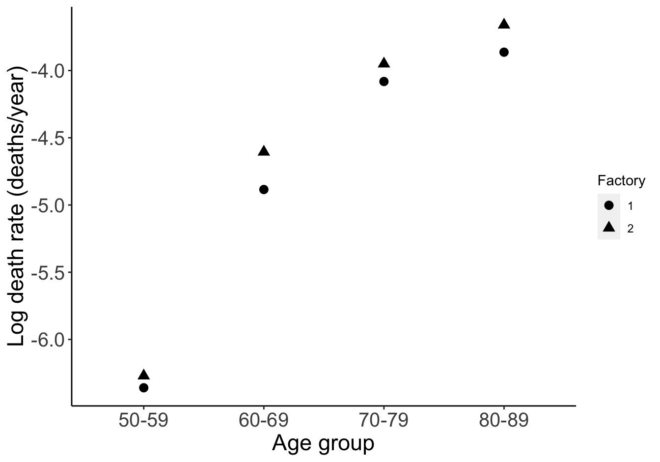

圖 62.1: Rates increase with age and age specific rates are higher in factory 2.

下面是 Stata 繪製圖62.2的代碼：

gen logdeathR = log(deaths/pyrs)
twoway (scatter logdeathR agegrp, name(deathRAge, replace) mlabel(factory)), xtitle(age group) xlabel (1(1)4.2)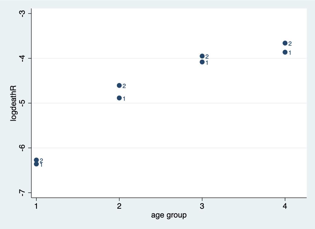

圖 62.2: Rates increase with age and age specific rates are higher in factory 2.

不論你用哪個圖，都可以看出，死亡率隨年齡增長而增加，2號工廠的死亡率似乎在各個年齡組都較1號工廠高。

62.6.3 請用數學語言描述死亡率和年齡組之間關係的模型。

令 \(Y_i\) 爲年齡組 \(i, (i = 1,\dots,8)\) 死亡人數，對應的觀測時間則爲 \(t_i\) 年。如果前提條件每名工人之間相互獨立可以認爲得到滿足，那麼 \(Y_i\) 可以用一個死亡率爲 \(\lambda_i\) 的泊松模型來描述：

\[ Y_i \sim \text{Po}(\mu_i) \text{ where } \mu_i = \lambda_i t_i \]

對應的鏈接方程以及其線性預測變量之間的關係可以表述爲：

\[ \begin{aligned} \eta_i & = \log(\mu_i) = \log(t_i) + \beta_0 + \beta_1x_{1i} + \beta_2x_{2i} + \beta_3x_{3i} \\ \text{where } x_{1i} & = \left\{ \begin{array}{ll} 0 \text{ if the } i \text{th group is not aged 60-69}\\ 1 \text{ if the } i \text{th group is aged 60-69}\\ \end{array} \right. \\ \text{where } x_{2i} & = \left\{ \begin{array}{ll} 0 \text{ if the } i \text{th group is not aged 70-79}\\ 1 \text{ if the } i \text{th group is aged 70-79}\\ \end{array} \right. \\ \text{where } x_{3i} & = \left\{ \begin{array}{ll} 0 \text{ if the } i \text{th group is not aged 80-89}\\ 1 \text{ if the } i \text{th group is aged 80-89}\\ \end{array} \right. \\ \end{aligned} \]

62.6.3.1 用R和Stata計算上述數學模型描述的死亡率和年齡之間關係的極大似然估計 (MLE)。年齡對於死亡率的效果有多強？

# fit a model without "agegroup"
mA <- glm(n_deaths ~ offset(log(Pyears)), 
              family = poisson(link = "log"), data = Rubber)
jtools::summ(mA, confint = TRUE, digits = 6)

Observations	8
Dependent variable	n_deaths
Type	Generalized linear model
Family	poisson
Link	log

𝛘²(0)	-0.000000
Pseudo-R² (Cragg-Uhler)	0.000000
Pseudo-R² (McFadden)	0.000000
AIC	142.725329
BIC	142.804771

	Est.	2.5%	97.5%	z val.	p
(Intercept)	-4.795015	-4.949964	-4.640067	-60.652699	0.000000
Standard errors: MLE

# fit a model with age group
mB <- glm(n_deaths ~ Agegrp + offset(log(Pyears)), 
              family = poisson(link = "log"), data = Rubber)
jtools::summ(mB, confint = TRUE, digits = 6)

Observations	8
Dependent variable	n_deaths
Type	Generalized linear model
Family	poisson
Link	log

𝛘²(3)	102.171839
Pseudo-R² (Cragg-Uhler)	0.999997
Pseudo-R² (McFadden)	0.726037
AIC	46.553491
BIC	46.871257

	Est.	2.5%	97.5%	z val.	p
(Intercept)	-6.315875	-6.839697	-5.792052	-23.631839	0.000000
Agegrp60-69	1.582833	1.004549	2.161118	5.364657	0.000000
Agegrp70-79	2.302963	1.725477	2.880448	7.816170	0.000000
Agegrp80-89	2.554674	1.847314	3.262034	7.078532	0.000000
Standard errors: MLE

lrtest(mA, mB)

## Likelihood ratio test
## 
## Model 1: n_deaths ~ offset(log(Pyears))
## Model 2: n_deaths ~ Agegrp + offset(log(Pyears))
##   #Df   LogLik Df   Chisq Pr(>Chisq)    
## 1   1 -70.3627                          
## 2   4 -19.2767  3 102.172 < 2.22e-16 ***
## ---
## Signif. codes:  0 '***' 0.001 '**' 0.01 '*' 0.05 '.' 0.1 ' ' 1

你可以比較加入年齡和沒加入年齡時的兩個模型，如上面使用的似然比檢驗法 (likelihood ratio test)。

在 Stata 你可以這樣做上面相同的事：

## 
## . infile agegrp factory deaths pyrs using "../backupfiles/RUBBER.RAW", clear
## (8 observations read)
## 
## . 
## . gen lpyrs = log(pyrs)
## 
## . 
## . glm deaths, family(poisson) offset(lpyrs) link(log)
## 
## Iteration 0:   log likelihood =  -76.82037  
## Iteration 1:   log likelihood = -70.363937  
## Iteration 2:   log likelihood = -70.362666  
## Iteration 3:   log likelihood = -70.362666  
## 
## Generalized linear models                         Number of obs   =          8
## Optimization     : ML                             Residual df     =          7
##                                                   Scale parameter =          1
## Deviance         =  103.8826147                   (1/df) Deviance =   14.84037
## Pearson          =  103.4540571                   (1/df) Pearson  =   14.77915
## 
## Variance function: V(u) = u                       [Poisson]
## Link function    : g(u) = ln(u)                   [Log]
## 
##                                                   AIC             =   17.84067
## Log likelihood   =  -70.3626661                   BIC             =   89.32652
## 
## ------------------------------------------------------------------------------
##              |                 OIM
##       deaths |      Coef.   Std. Err.      z    P>|z|     [95% Conf. Interval]
## -------------+----------------------------------------------------------------
##        _cons |  -4.795015   .0790569   -60.65   0.000    -4.949964   -4.640067
##        lpyrs |          1  (offset)
## ------------------------------------------------------------------------------
## 
## . est store A
## 
## . 
## . glm deaths i.agegrp, family(poisson) offset(lpyrs) link(log)
## 
## Iteration 0:   log likelihood = -19.667375  
## Iteration 1:   log likelihood = -19.277924  
## Iteration 2:   log likelihood = -19.276748  
## Iteration 3:   log likelihood = -19.276748  
## 
## Generalized linear models                         Number of obs   =          8
## Optimization     : ML                             Residual df     =          4
##                                                   Scale parameter =          1
## Deviance         =  1.710778974                   (1/df) Deviance =   .4276947
## Pearson          =  1.704679988                   (1/df) Pearson  =     .42617
## 
## Variance function: V(u) = u                       [Poisson]
## Link function    : g(u) = ln(u)                   [Log]
## 
##                                                   AIC             =   5.819187
## Log likelihood   = -19.27674826                   BIC             =  -6.606987
## 
## ------------------------------------------------------------------------------
##              |                 OIM
##       deaths |      Coef.   Std. Err.      z    P>|z|     [95% Conf. Interval]
## -------------+----------------------------------------------------------------
##       agegrp |
##           2  |   1.582834   .2950484     5.36   0.000     1.004549    2.161118
##           3  |   2.302963   .2946408     7.82   0.000     1.725477    2.880448
##           4  |   2.554674   .3609046     7.08   0.000     1.847314    3.262034
##              |
##        _cons |  -6.315874   .2672612   -23.63   0.000    -6.839697   -5.792052
##        lpyrs |          1  (offset)
## ------------------------------------------------------------------------------
## 
## . est store B
## 
## . 
## . lrtest A B
## 
## Likelihood-ratio test                                 LR chi2(3)  =    102.17
## (Assumption: A nested in B)                           Prob > chi2 =    0.0000
## 
## .

其實Stata裏面還可以用簡化的 Poisson 命令

## 
## . infile agegrp factory deaths pyrs using "../backupfiles/RUBBER.RAW", clear
## (8 observations read)
## 
## . 
## . gen lpyrs = log(pyrs)
## 
## . 
## . poisson deaths i.agegrp, e(pyrs)
## 
## Iteration 0:   log likelihood = -19.280832  
## Iteration 1:   log likelihood = -19.276746  
## Iteration 2:   log likelihood = -19.276745  
## 
## Poisson regression                              Number of obs     =          8
##                                                 LR chi2(3)        =     102.17
##                                                 Prob > chi2       =     0.0000
## Log likelihood = -19.276745                     Pseudo R2         =     0.7260
## 
## ------------------------------------------------------------------------------
##       deaths |      Coef.   Std. Err.      z    P>|z|     [95% Conf. Interval]
## -------------+----------------------------------------------------------------
##       agegrp |
##           2  |   1.582833   .2950484     5.36   0.000     1.004549    2.161118
##           3  |   2.302962   .2946408     7.82   0.000     1.725477    2.880448
##           4  |   2.554674   .3609046     7.08   0.000     1.847314    3.262034
##              |
##        _cons |  -6.315874   .2672612   -23.63   0.000    -6.839697   -5.792052
##     ln(pyrs) |          1  (exposure)
## ------------------------------------------------------------------------------
## 
## .

62.6.3.2 計算下列兩組年齡組對比之下的模型估計死亡率比 (rate ratios)

60-69歲比 50-59歲 RR 及其 95%CI

\[ \exp(1.583) (\exp(1.005), \exp(2.161)) = 4.87 (2.73, 8.68) \]

80-89歲比 70-79歲 RR 及其 95%CI 的計算

\[ \exp(\hat{\beta_3} - \hat{\beta_2}) = \exp(2.555 - 2.302) = 1.29 \]

爲了獲取 \(\hat{\beta_3} - \hat{\beta_2}\) 的方差，已知 \(\text{Var}(\hat{\beta_3} - \hat{\beta_2}) = \text{Var}(\hat{\beta_3}) + \text{Var}(\hat{\beta_2}) - 2\text{Cov}(\hat{\beta_3}, \hat{\beta_2})\)。根據這個在概率論學到的方差性質，我們可以手動計算想要的方差和標準差，從而進一步獲取其 95% CI：

You can also use vce command in Stata to obtain the Covariance matrix of coefficients of a fitted poisson model

vcov(mB)

##              (Intercept)  Agegrp60-69  Agegrp70-79  Agegrp80-89
## (Intercept)  0.071428571 -0.071428571 -0.071428571 -0.071428571
## Agegrp60-69 -0.071428571  0.087053571  0.071428571  0.071428571
## Agegrp70-79 -0.071428571  0.071428571  0.086813187  0.071428571
## Agegrp80-89 -0.071428571  0.071428571  0.071428571  0.130252101

\[ \begin{aligned} \text{Var}(\hat{\beta_3} - \hat{\beta_2}) & = \text{Var}(\hat{\beta_3}) + \text{Var}(\hat{\beta_2}) - 2\text{Cov}(\hat{\beta_3}, \hat{\beta_2}) \\ & = 0.13025 + 0.08681 - 2 \times 0.07143 \\ & = 0.0743 \\ \Rightarrow \text{the 95%CI} & = \exp(2.555 - 2.303 \pm\sqrt{0.07143}) \\ & = (0.75, 2.20) \end{aligned} \]

在R裏你可以這樣計算：

# change the reference group to "70-79"
Rubber <- Rubber %>% 
  mutate(Agegrp1 = fct_relevel(Agegrp, "70-79"))

mC <- glm(n_deaths ~ Agegrp1 + offset(log(Pyears)), 
              family = poisson(link = "log"), data = Rubber)
jtools::summ(mC, confint = TRUE, digits = 6, exp = TRUE)

Observations	8
Dependent variable	n_deaths
Type	Generalized linear model
Family	poisson
Link	log

𝛘²(3)	102.171839
Pseudo-R² (Cragg-Uhler)	0.999997
Pseudo-R² (McFadden)	0.726037
AIC	46.553491
BIC	46.871257

	exp(Est.)	2.5%	97.5%	z val.	p
(Intercept)	0.018081	0.014179	0.023056	-32.353131	0.000000
Agegrp150-59	0.099962	0.056110	0.178088	-7.816170	0.000000
Agegrp160-69	0.486689	0.344635	0.687297	-4.089424	0.000043
Agegrp180-89	1.286225	0.754119	2.193786	0.924013	0.355480
Standard errors: MLE

但是在 Stata 裏面可以使用靈活無比的 lincom 命令：

## 
## . infile agegrp factory deaths pyrs using "../backupfiles/RUBBER.RAW", clear
## (8 observations read)
## 
## . 
## . gen lpyrs = log(pyrs)
## 
## . 
## . quietly: poisson deaths i.agegrp, e(pyrs)
## 
## . lincom 4.agegrp - 3.agegrp, eform
## 
##  ( 1)  - [deaths]3.agegrp + [deaths]4.agegrp = 0
## 
## ------------------------------------------------------------------------------
##       deaths |     exp(b)   Std. Err.      z    P>|z|     [95% Conf. Interval]
## -------------+----------------------------------------------------------------
##          (1) |   1.286225   .3503829     0.92   0.355     .7541189    2.193786
## ------------------------------------------------------------------------------
## 
## .

62.6.4 接下來的模型中在前面的基礎上加入工廠編號，你認爲是否有證據證明工廠之間的工人的死亡率在調整了年齡之後依然有差異？計算年齡調整過後的兩工廠之間死亡率之比和95%CI。

mD <- glm(n_deaths ~ Agegrp + Factory + offset(log(Pyears)), 
              family = poisson(link = "log"), data = Rubber)
jtools::summ(mD, confint = TRUE, digits = 6, exp = TRUE)

Observations	8
Dependent variable	n_deaths
Type	Generalized linear model
Family	poisson
Link	log

𝛘²(4)	103.666936
Pseudo-R² (Cragg-Uhler)	0.999998
Pseudo-R² (McFadden)	0.736662
AIC	47.058393
BIC	47.455601

	exp(Est.)	2.5%	97.5%	z val.	p
(Intercept)	0.001640	0.000947	0.002839	-22.900655	0.000000
Agegrp60-69	4.839413	2.714014	8.629254	5.343443	0.000000
Agegrp70-79	9.949876	5.584586	17.727369	7.796966	0.000000
Agegrp80-89	12.864610	6.341532	26.097509	7.077995	0.000000
Factory2	1.213953	0.888998	1.657687	1.219745	0.222561
Standard errors: MLE

lrtest(mD, mB)

## Likelihood ratio test
## 
## Model 1: n_deaths ~ Agegrp + Factory + offset(log(Pyears))
## Model 2: n_deaths ~ Agegrp + offset(log(Pyears))
##   #Df   LogLik Df  Chisq Pr(>Chisq)
## 1   5 -18.5292                     
## 2   4 -19.2767 -1 1.4951    0.22143

從 mD 模型的報告來看，2號工廠比較1號工廠的工人死亡率比是 1.21 (95%CI: 0.89, 1.66)。兩個模型的似然比檢驗結果也提示，並無確實證據證明兩工廠工人的死亡率在調整了年齡因素之後有顯著差異。

62.6.5 現在在前一步加了工廠變量的基礎上，重新擬合模型，加入工廠和年齡之間的交互作用項

mE <- glm(n_deaths ~ Agegrp + Factory + Factory*Agegrp 
                    + offset(log(Pyears)), 
              family = poisson(link = "log"), data = Rubber)
summary(mE); jtools::summ(mE, confint = TRUE, digits = 6, exp = TRUE)

## 
## Call:
## glm(formula = n_deaths ~ Agegrp + Factory + Factory * Agegrp + 
##     offset(log(Pyears)), family = poisson(link = "log"), data = Rubber)
## 
## Deviance Residuals: 
## [1]  0  0  0  0  0  0  0  0
## 
## Coefficients:
##                       Estimate Std. Error  z value  Pr(>|z|)    
## (Intercept)          -6.359327   0.377964 -16.8252 < 2.2e-16 ***
## Agegrp60-69           1.474563   0.424139   3.4766 0.0005078 ***
## Agegrp70-79           2.277842   0.419750   5.4267 5.742e-08 ***
## Agegrp80-89           2.495969   0.517549   4.8227 1.416e-06 ***
## Factory2              0.088878   0.534522   0.1663 0.8679394    
## Agegrp60-69:Factory2  0.190175   0.591421   0.3216 0.7477889    
## Agegrp70-79:Factory2  0.042462   0.589592   0.0720 0.9425869    
## Agegrp80-89:Factory2  0.113771   0.722375   0.1575 0.8748544    
## ---
## Signif. codes:  0 '***' 0.001 '**' 0.01 '*' 0.05 '.' 0.1 ' ' 1
## 
## (Dispersion parameter for poisson family taken to be 1)
## 
##     Null deviance: 1.03883e+02  on 7  degrees of freedom
## Residual deviance: 1.04361e-14  on 0  degrees of freedom
## AIC: 52.8427
## 
## Number of Fisher Scoring iterations: 3

Observations	8
Dependent variable	n_deaths
Type	Generalized linear model
Family	poisson
Link	log

𝛘²(7)	103.882612
Pseudo-R² (Cragg-Uhler)	0.999998
Pseudo-R² (McFadden)	0.738194
AIC	52.842718
BIC	53.478250

	exp(Est.)	2.5%	97.5%	z val.	p
(Intercept)	0.001731	0.000825	0.003630	-16.825197	0.000000
Agegrp60-69	4.369124	1.902683	10.032807	3.476599	0.000508
Agegrp70-79	9.755607	4.285111	22.209899	5.426658	0.000000
Agegrp80-89	12.133483	4.399941	33.459862	4.822670	0.000001
Factory2	1.092948	0.383366	3.115916	0.166276	0.867939
Agegrp60-69:Factory2	1.209461	0.379467	3.854873	0.321556	0.747789
Agegrp70-79:Factory2	1.043376	0.328533	3.313620	0.072019	0.942587
Agegrp80-89:Factory2	1.120495	0.271972	4.616327	0.157495	0.874854
Standard errors: MLE

62.6.5.1 請問這是一個怎樣的模型？

這是一個有8組觀測數據，8個參數估計的模型，是一個飽和模型。 The model is saturated.

62.6.5.2 有沒有足夠的證據證明工廠和年齡變量之間的交互作用項是有意義的？

lrtest(mE, mD)

## Likelihood ratio test
## 
## Model 1: n_deaths ~ Agegrp + Factory + Factory * Agegrp + offset(log(Pyears))
## Model 2: n_deaths ~ Agegrp + Factory + offset(log(Pyears))
##   #Df   LogLik Df   Chisq Pr(>Chisq)
## 1   8 -18.4214                      
## 2   5 -18.5292 -3 0.21568    0.97502

似然比檢驗結果顯示，沒有證據證明二者之間交互作用項是有意義的。

62.6.5.3 用數學語言描述上述包含了交互作用項的模型，並利用這個模型手頭計算下列各組的死亡率：

1號工廠的 70-79 歲
2號工廠的 50-50 歲
2號工廠的 60-69 歲

\[ \begin{aligned} \eta_i = \log(\mu_i) & = \log(t_i) + \beta_0 + \beta_1x_{1i} + \beta_2x_{2i} + \beta_3x_{3i} + \beta_4z_{i} \\ & \;\;\; + \beta_5(x_{1i}z_{i}) + \beta_6(x_{2i}z_{i}) + \beta_7(x_{3i}z_{i})\\ \text{where } x_{1i} & = \left\{ \begin{array}{ll} 0 \text{ if the } i \text{th group is not aged 60-69}\\ 1 \text{ if the } i \text{th group is aged 60-69}\\ \end{array} \right. \\ \text{where } x_{2i} & = \left\{ \begin{array}{ll} 0 \text{ if the } i \text{th group is not aged 70-79}\\ 1 \text{ if the } i \text{th group is aged 70-79}\\ \end{array} \right. \\ \text{where } x_{3i} & = \left\{ \begin{array}{ll} 0 \text{ if the } i \text{th group is not aged 80-89}\\ 1 \text{ if the } i \text{th group is aged 80-89}\\ \end{array} \right. \\ \text{and } z_{i} & = \left\{ \begin{array}{ll} 0 \text{ if the } i \text{th group is from factory 1}\\ 1 \text{ if the } i \text{th group is from factory 2}\\ \end{array} \right. \end{aligned} \]

1號工廠的 70-79 歲組中該模型估計的死亡率是

\[ \exp(\hat{\beta}_0 + \hat{\beta}_2) = \exp(-6.359 + 2.2778) = 16.9 /1000 \text{ person-years} \]

2號工廠的 50-59 歲組中該模型估計的死亡率是

\[ \exp(\hat{\beta}_0 + \hat{\beta}_4) = \exp(-6.359 + 0.089) = 1.89 / 1000 \text{ person-years} \]

2號工廠的 60-69 歲組中該模型估計的死亡率是

\[ \exp(\hat{\beta}_0 + \hat{\beta}_1 + \hat{\beta}_4 + \hat{\beta}_5) = \exp(-6.359 + 1.475 + 0.089 + 0.190) = 10.0 / 1000 \text{ person-years} \]

62.6.5.4 對比你計算的模型估計死亡率和實際觀測到的死亡率

tab <- stat.table(index=list(Factory=Factory,Agegrp=Agegrp),
                   contents=list(sum(n_deaths/Pyears)), 
                  data=Rubber, margins=FALSE)

print(tab, digits = 7)

##  -------------------------------------------------- 
##           -----------------Agegrp------------------ 
##  Factory       50-59     60-69     70-79     80-89  
##  -------------------------------------------------- 
##  1         0.0017305 0.0075609 0.0168824 0.0209974  
##  2         0.0018914 0.0099946 0.0192519 0.0257143  
##  --------------------------------------------------

我們發現該模型估計的各組的死亡率和觀測值完全一致。

62.6.6 現在把年齡當作連續型變量來考慮。擬合下列模型

62.6.6.1 只有年齡作爲連續型變量

mF <- glm(n_deaths ~ as.numeric(Agegrp) + offset(log(Pyears)), 
              family = poisson(link = "log"), data = Rubber)
jtools::summ(mF, confint = TRUE, digits = 6, exp = TRUE)

Observations	8
Dependent variable	n_deaths
Type	Generalized linear model
Family	poisson
Link	log

𝛘²(1)	89.442531
Pseudo-R² (Cragg-Uhler)	0.999986
Pseudo-R² (McFadden)	0.635582
AIC	55.282799
BIC	55.441682

	exp(Est.)	2.5%	97.5%	z val.	p
(Intercept)	0.001421	0.000910	0.002217	-28.874573	0.000000
as.numeric(Agegrp)	2.239658	1.899333	2.640963	9.588396	0.000000
Standard errors: MLE

mF 的結果提供很強的證據證明年齡作爲連續型變量和死亡率的變化有關。年齡每增加10歲，死亡率增長的數字要乘以 2.24。

62.6.6.2 年齡和工廠兩個預測變量

mG <- glm(n_deaths ~ as.numeric(Agegrp) + Factory + offset(log(Pyears)), 
              family = poisson(link = "log"), data = Rubber)
jtools::summ(mG, confint = TRUE, digits = 6, exp = TRUE)

Observations	8
Dependent variable	n_deaths
Type	Generalized linear model
Family	poisson
Link	log

𝛘²(2)	91.170538
Pseudo-R² (Cragg-Uhler)	0.999989
Pseudo-R² (McFadden)	0.647862
AIC	55.554792
BIC	55.793116

	exp(Est.)	2.5%	97.5%	z val.	p
(Intercept)	0.001274	0.000790	0.002053	-27.358186	0.000000
as.numeric(Agegrp)	2.239890	1.899067	2.641880	9.575477	0.000000
Factory2	1.231652	0.902034	1.681716	1.311155	0.189805
Standard errors: MLE

lrtest(mG, mF)

## Likelihood ratio test
## 
## Model 1: n_deaths ~ as.numeric(Agegrp) + Factory + offset(log(Pyears))
## Model 2: n_deaths ~ as.numeric(Agegrp) + offset(log(Pyears))
##   #Df   LogLik Df   Chisq Pr(>Chisq)
## 1   3 -24.7774                      
## 2   2 -25.6414 -1 1.72801    0.18867

並無有效證據證明工廠之間有死亡率的顯著區別。

62.6.6.3 年齡和工廠，及兩個變量的交互作用項

mH <- glm(n_deaths ~ as.numeric(Agegrp) + Factory  + as.numeric(Agegrp)*Factory + 
          offset(log(Pyears)), family = poisson(link = "log"), data = Rubber)
jtools::summ(mH, confint = TRUE, digits = 6, exp = TRUE)

Observations	8
Dependent variable	n_deaths
Type	Generalized linear model
Family	poisson
Link	log

𝛘²(3)	91.183730
Pseudo-R² (Cragg-Uhler)	0.999989
Pseudo-R² (McFadden)	0.647955
AIC	57.541599
BIC	57.859365

	exp(Est.)	2.5%	97.5%	z val.	p
(Intercept)	0.001240	0.000642	0.002395	-19.936299	0.000000
as.numeric(Agegrp)	2.263303	1.776141	2.884084	6.605055	0.000000
Factory2	1.293657	0.528919	3.164090	0.564224	0.572602
as.numeric(Agegrp):Factory2	0.980790	0.704402	1.365623	-0.114855	0.908560
Standard errors: MLE

lrtest(mG, mH)

## Likelihood ratio test
## 
## Model 1: n_deaths ~ as.numeric(Agegrp) + Factory + offset(log(Pyears))
## Model 2: n_deaths ~ as.numeric(Agegrp) + Factory + as.numeric(Agegrp) * 
##     Factory + offset(log(Pyears))
##   #Df   LogLik Df   Chisq Pr(>Chisq)
## 1   3 -24.7774                      
## 2   4 -24.7708  1 0.01319    0.90856

並無有效證據證明工廠之間的相互作用項有意義。

62.6.7 計算只有年齡(連續型)和工廠兩個變量模型時的模型偏差 (deviance)，該模型和第一部分中飽和模型之間相比相差幾個參數(parameters)？你有怎樣的推論？

lrtest(mF, mE)

## Likelihood ratio test
## 
## Model 1: n_deaths ~ as.numeric(Agegrp) + offset(log(Pyears))
## Model 2: n_deaths ~ Agegrp + Factory + Factory * Agegrp + offset(log(Pyears))
##   #Df   LogLik Df   Chisq Pr(>Chisq)  
## 1   2 -25.6414                        
## 2   8 -18.4214  6 14.4401   0.025088 *
## ---
## Signif. codes:  0 '***' 0.001 '**' 0.01 '*' 0.05 '.' 0.1 ' ' 1

看上面似然比檢驗結果顯示，有一些不太強的證據 (p = 0.0262) 證明相對飽和模型來說，把年齡當連續變量的模型可能擬合度較差。所以把年齡當作分類型變量 (categorical) 會是比較好的選擇。

62.6.8 對這個數據進行了這一系列的分析之後，你從流行病學的角度來說，有怎樣的結論？

總的來說，死亡率隨着年齡增長而增加。60-69 歲組的死亡率是50-59 歲組的 4.8 (95% CI 2.7, 8.6) 倍。之後年齡每增長十歲死亡率也在增長，只是增長幅度逐漸減少。至於工廠之間的死亡率比較，2號工廠似乎有 21% 較高 (95%CI: -11%, 66%) 的死亡率。但是工廠之間的死亡率差異並無顯著性 (p = 0.22)。交互作用項的分析也表明，並沒有證據表明工廠之間的死亡率差異會由於年齡的變化而有所不同。

第 62 章 率的廣義線性迴歸 Poisson GLM for rates