第 63 章 混雜的調整，交互作用，和模型的可壓縮性

臨牀醫學，流行病學研究的許多問題，需要我們通過數據來評估某些結果變量 (outcome) 和某些預測變量 (predictors/exposures) 之間的關係 (甚至是因果關係)。這些問題的最佳解決方法應該說是隨機臨牀試驗 (ramdomized clinical trial, RCT)。但是有更多的時候 (由於違反醫學倫理，或者現狀所困，甚至是知識有限) 我們無法設計 RCT 來解決這些問題，就只能藉助於觀察性研究 (observational study)。觀察性研究最大的侷限性在於無法像 RCT 那樣從實驗設計階段把混雜因素排除或者降到最低，所以觀察數據在分析的時候，混雜 (confounding) 是必須要加以考慮的一大要因。在簡單線性迴歸章節 (Section 30.5)，詳細討論過混雜因素的定義及條件：

對於一個預測變量是否夠格被叫做混雜因子，它必須滿足下面的條件：

• 與關心的預測變量相關 (i.e. \(\delta_1 \neq 0\))；
• 與因變量相關 (當關心的預測變量不變時，\(\beta_2\neq0\) )；
• 不在預測變量和因變量的因果關係 (如果有的話) 中作媒介。Not be on the causal pathway between the predictor of interest and the dependent variable.

下面的統計數據來自一個比較手術和超聲碎石術對於腎結石治療結果的評價。已知大多數醫生都公認，腎結石的直徑小於 2 公分時治療成功的概率較高。

表 63.1: Lithotripsy

	< 2cm Diameter		>= 2cm Diameter
Group	Surgery	Lithotripsy	Surgery	Lithotripsy
Success	81.00	234	192.00	55
Failure	6.00	36	71.00	25
Total	87.00	270	263.00	80
Odds Ratios	2.08		1.23

可以看到，在上面的分組表格中，左右兩邊的四格表分別統計了腎結石尺寸小於 2 cm 和大於 2 cm 時，手術摘除腎結石的成功/失敗次數，以及超聲碎石術的成功/失敗次數。這個表格告訴我們，無論腎結石的尺寸是大於還是小於 2 cm，手術的成功的比值比都大於超聲碎石術。但是如果我們沒有把數據按照腎結石尺寸區分時，數據就被壓縮 (collapsed) 成了下面表格總結的樣子：

表 63.2: Lithotripsy data collapsed

Outcome	Surgery	Lithotripsy
Success	273 (78%)	289 (83%)
Failure	77	61
Total	350	350
Odds ratio	0.75

當腎結石尺寸被忽略時，數據卻顯示超聲碎石術的成功比值比要高於手術，和之前的結果是矛盾的，你會信哪個？

不要慌，數據不會撒謊，撒謊(有意掩蓋事實)的永遠是人類。我們來把手術次數，超聲碎石術次數，以及腎結石尺寸之間的關係再列個表格：

表 49.3: Association between treatment and the size of the stone.

Size of the Stone	Surgery	Lithotripsy
\(< 2\) cm	87 (33%)	270 (77%)
\(\geqslant 2\) cm	263	80
Total	350	350

可見醫生也都不是傻子，明明腎結石尺寸很大還要用超聲碎石術的人很少，有 77% 的腎結石尺寸小的患者選擇了超聲碎石術。然後我們再列一個表格來看看腎結石的尺寸大小和超聲碎石術成功與否有沒有關係：

表 49.4: Among the lithotripsy patients higher percentage of success was observed when stones were small.

Outcome	\(< 2\) cm	\(\geqslant 2\) cm
Success	234 (87%)	55 (69%)
Failure	36	25
Total	370	80

可見結石尺寸較大時，超聲碎石術的成功率 (69%)，明顯低於尺寸小的時候的成功率 (87%)。在選擇做外科手術的患者中，大多數人的結石尺寸大於 2 cm，成功率仍然達到了 73%。

表 49.5: Among the surgery patients higher percentage of success in both stones compared with lithotripsy

Outcome	\(< 2\) cm	\(\geqslant 2\) cm
Success	81 (93%)	192 (73%)
Failure	6	71
Total	87	263

看到這裏，你是否也發現了，腎結石尺寸大小，同時和手術類型的選擇有關 (尺寸小的傾向於選擇超聲碎石術)，尺寸大小，同樣也和手術結果的成功與否，高度相關 (結石小的人成功率高)。所以，分析手術類型和結石手術的成功率的關係的時候，患者體內結石尺寸的大小，對這個關係是產生了混雜效應的。他們三者之間的關係，可以用下面的圖 63.1 來理解：

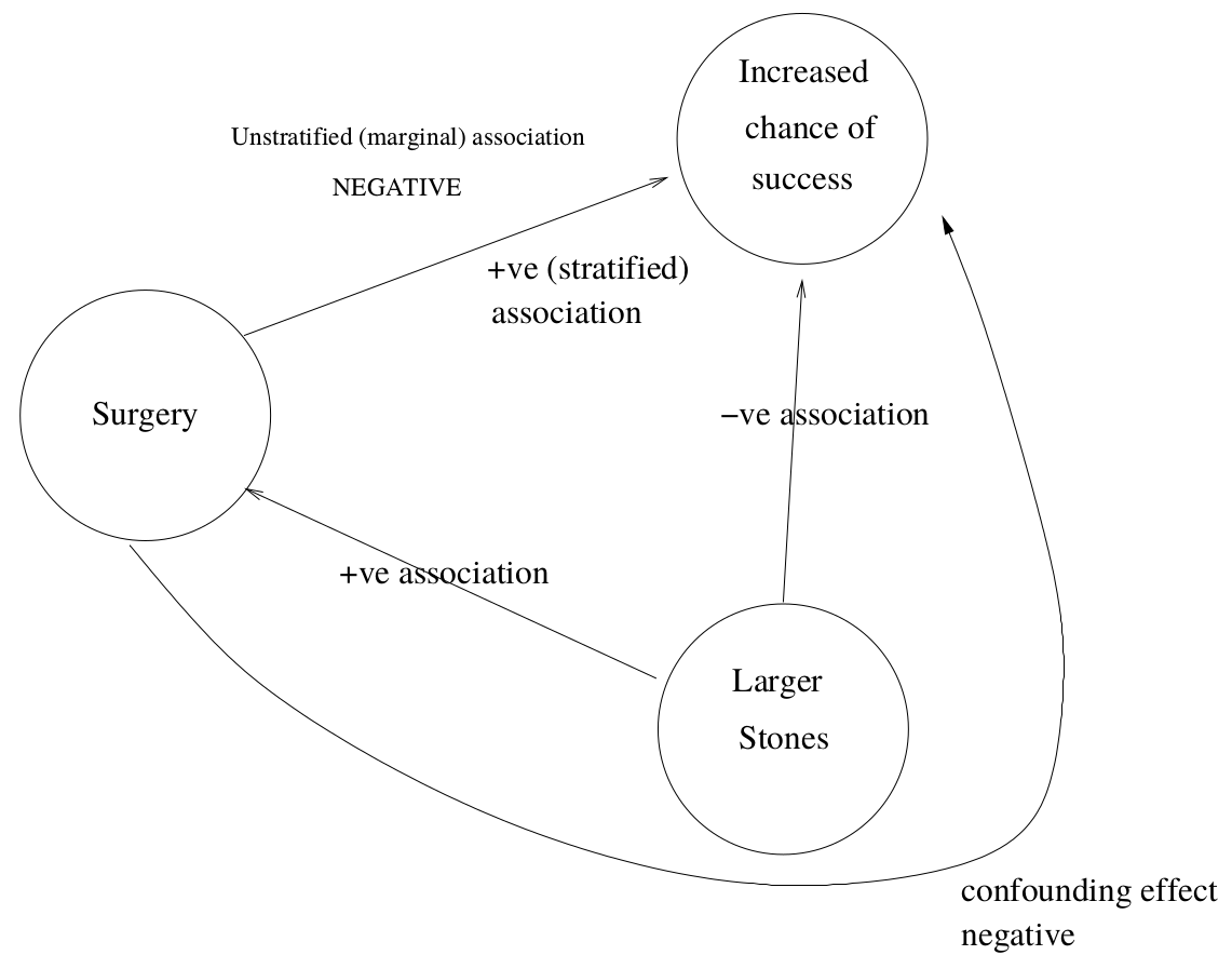
圖 63.1: Confounding in kidney stones example

當數據被壓縮 (忽略了腎結石尺寸時)，比較兩種手術類型的成功率的時候，接受外科手術患者的尺寸大多數都較大的事實被“人爲的掩蓋住了”，但是當數據按照結石大小分層以後，你會看見外科手術不論是對付大的結石，還是小的結石，成功率都高於超聲碎石術。這個例子是混雜效應直接逆轉真實相關關係的極佳的實例。同時也提示我們，總體的比值比 (overall odds ratio) 不能通過簡單地把分層表格直接壓縮 (collapsed table) 獲得的數字來計算。

63.1 混雜因素的調整

在前面的腎結石手術的例子中，我們利用已有的背景知識 (小尺寸結石的成功率高)，和初步的統計分析 (變量之間兩兩列表分析其內在關係) 發現了混雜因素 (結石尺寸)，並且其結果也讓我們認定了要暴露因素和結果變量之間的關係，混雜因素必須被調整 (adjusted)。

如腎結石數據這樣簡單的情境下 (被認爲是混雜因素的變量和預測變量/暴露變量都只是一個二進制變量)，我們可以把變量兩兩捉對列表分析其相互關係，確定了混雜效應以後把暴露變量和結果變量按照混雜因素的有無列表之後，就可以求得混雜因素被調整後的分層的比值比。這些分層比值比，在暴露變量與結果變量的關係保持混雜因素的層之間保持不變的前提下，可以被“平均化”(簡單地說)以後求得總體/合併的比值比 (overall/pooled odds ratio)。這就是 Mantel-Haenszel 法或者 Woolf 法的合併比值比的思想出發點。我們來回顧一下 Woolf 法的全部計算過程：

現在假設我們關心的是某種疾病的患病與否 (是/否)，和某個暴露變量 (是/否) 之間的關係，但是同時想要調整另一個具有 \(k\) 個分層的混雜因素變量。

表 49.6: Woolf Method for estimating the stratified and pooled odds ratio

		Group
		\(X=0\)	\(X=1\)
\(D=0\)	\(X=0\)	\(n_{00}\)	\(n_{10}\)
	\(X=1\)	\(n_{01}\)	\(n_{10}\)

63.1.1 Woolf 法估算合併比值比

對想要調整的一個 \(k\) 組的混雜因素，把數據按照它的分組分層整理以後，可以得到上面的 \(k\) 個四格表 (每個分層四格表都是暴露變量和結果變量結合的四個觀察值 \(a_i, b_i, c_i, d_i, (i=1,\cdots, k)\))。每個分層四格表的觀測比值比爲 \(\hat\Psi_i = \frac{a_id_i}{c_ib_i}\)，且可以證明方差爲

\[ \text{Var}(\text{log}\hat\Psi_i) \approx \frac{1}{a_i} + \frac{1}{b_i} + \frac{1}{c_i} + \frac{1}{d_i} = \frac{1}{w_i} \]

合併比值比的對數 \(\text{log}\hat\Psi_w\) 的 Woolf 的計算方法就是

\[ \text{log}\hat\Psi_w = \frac{\sum w_i\text{log}\hat\Psi_i}{\sum w_i} \]

所以，每個分層的對數比值比乘以自己的方差的倒數 (權重 weights) 之後求和，再除以所有權重之和，獲得的是合併後的對數比值比，然後再逆運算回來就是 Woolf 法計算合併比值比的原理是。

這個合併比值比的對數的方差是

\[ \text{Var}(\text{log}\hat\Psi_w) = \frac{1}{\sum w_i} \]

有了加權後的合併比值比，和方差，就可以求加權後的合併比值比的信賴區間了。值得注意的是，分層之後每個分層四格表中的四個數字 (四個樣本量) 都不能太小。腎結石手術數據滿足這些條件，那麼不妨跟我一起手算一下結石尺寸調整後的手術與超聲碎石術成功與否的比值比：

\[ \begin{aligned} \hat\Psi_1 = 2.08 ;&\; \hat\Psi_2 = 1.23 \\ \text{Var}(\text{log}\hat\Psi_1) = \frac{1}{81} & + \frac{1}{234} + \frac{1}{6} + \frac{1}{36} = 0.2111 \\ \text{Var}(\text{log}\hat\Psi_2) = \frac{1}{192} & + \frac{1}{55} + \frac{1}{71} + \frac{1}{25} = 0.0775 \\ w_1 = \frac{1}{\text{Var}(\text{log}\hat\Psi_1)} = 4.74 ; \;& w_2 = \frac{1}{\text{Var}(\text{log}\hat\Psi_2)} = 12.91 \\ \text{log}\hat\Psi_w = & \frac{4.74\times\text{log(2.08)} + 12.91\times\text{log(1.23)}}{4.74 + 12.91} \\ = & 0.3481 \\ \Rightarrow \hat\Psi_w =& e^{0.3481} = 1.42\\ \text{Var}(\hat\Psi_w) =& \frac{1}{4.74+12.91} = 0.0567 \\ \Rightarrow 95\% \text{ CI} = & e^{0.3481 \pm 1.96\times\sqrt{0.0567}} \\ = & (0.89, 2.26) \end{aligned} \]

Woolf 的計算調整後的合併比值比的方法是在線性迴歸和廣義線性迴歸被發現之前誕生的，但是其想法之精妙，確實令人感嘆。可惜其最大的缺陷是無法用這樣的方法進行連續型變量的調整，也很難同時進行多個變量的調整，所以現在這一算法已經逐漸被淘汰。現在我們有了廣義線性迴歸模型這一更強大的工具，只要把變量加入廣義線性模型進行調整就可以計算曾經難以計算和擴展的調整後的合併比值比。從下面的代碼計算獲得的調整後比值比 \(1.43 (0.91, 2.34)\) 也可以看出，Woolf 方法的計算結果也是足夠令人滿意的。

size <- c("< 2cm", "< 2cm", ">= 2cm", ">= 2cm")
treatment <- c("Surgery","Lithotripsy","Surgery","Lithotripsy")
n <- c(87, 270, 263, 80)
Success <- c(81, 234, 192, 55)
Stone <- data.frame(size, treatment, n, Success)
ModelStone <- glm(cbind(Success, n - Success) ~ treatment + size, 
                  family = binomial(link = logit), data = Stone)
summary(ModelStone)

## 
## Call:
## glm(formula = cbind(Success, n - Success) ~ treatment + size, 
##     family = binomial(link = logit), data = Stone)
## 
## Deviance Residuals: 
##        1         2         3         4  
##  0.76357  -0.35881  -0.27563   0.46948  
## 
## Coefficients:
##                  Estimate Std. Error z value  Pr(>|z|)    
## (Intercept)       1.93655    0.17045 11.3614 < 2.2e-16 ***
## treatmentSurgery  0.35723    0.22908  1.5594    0.1189    
## size>= 2cm       -1.26057    0.23900 -5.2742 1.333e-07 ***
## ---
## Signif. codes:  0 '***' 0.001 '**' 0.01 '*' 0.05 '.' 0.1 ' ' 1
## 
## (Dispersion parameter for binomial family taken to be 1)
## 
##     Null deviance: 33.12395  on 3  degrees of freedom
## Residual deviance:  1.00816  on 1  degrees of freedom
## AIC: 26.3554
## 
## Number of Fisher Scoring iterations: 3

broom::tidy(ModelStone, exp = FALSE, conf.int = TRUE) %>% 
  knitr::kable(.)

term	estimate	std.error	statistic	p.value	conf.low	conf.high
(Intercept)	1.93655073	0.17044973	11.3614184	0.00000000	1.61463718	2.28439560
treatmentSurgery	0.35722866	0.22907985	1.5594068	0.11890013	-0.09069343	0.80856158
size>= 2cm	-1.26056536	0.23900383	-5.2742474	0.00000013	-1.73744172	-0.79909943

所以，此次分析的結論是，在 5% 的顯著性水平下，數據無法提供有效證據證明，當調整了結石尺寸之後，外科手術和超聲碎石術治療腎結石有差別。 We can conclude that there is no evidence at the 5% level for an effect of surgery, adjusted for stone size.

63.2 交互作用

我們決定調整一個混雜因素的時候，其實同時包含了 “在不同混雜因素的程度下，暴露變量和結果變量之間的關係不變/This implicitly assumes that the effect of the exposure is the same irrespective of the levels of the confounder.” 的假設。但是，一個混雜因素，它可能同時還扮演了改變暴露變量和結果變量之間關係的角色 (effect modifier/交互作用效應)。另外還有的情況下，某變量可能改變了暴露變量和結果變量之間的關係，卻不一定是一個混雜因素。此時我們說這個起到改變關係的變量和暴露變量之間發生了交互作用。

如果暴露變量在某個分組變量的不同層 (strata) 之間是不同質的 (hetergeneous, not constant)，我們建議要分析且報告不同層各自的比值比。惟一的例外是 RCT 臨牀試驗的時候，我們更加關心調整後合併比值比。因爲一項治療藥物對不同的 “個體” 有不同的療效是必然的，但是，RCT 的目的是要評價的其實是這個藥物或者新療法在整個人羣中的療效是怎樣的。

我們給腎結石數據加上治療方案和結石尺寸大小的交互作用項，結果如下：

ModelStone2 <- glm(cbind(Success, n - Success) ~ treatment*size, 
                   family = binomial(link = logit), data = Stone)
summary(ModelStone2)

## 
## Call:
## glm(formula = cbind(Success, n - Success) ~ treatment * size, 
##     family = binomial(link = logit), data = Stone)
## 
## Deviance Residuals: 
## [1]  0  0  0  0
## 
## Coefficients:
##                             Estimate Std. Error z value  Pr(>|z|)    
## (Intercept)                  1.87180    0.17903 10.4553 < 2.2e-16 ***
## treatmentSurgery             0.73089    0.45942  1.5909 0.1116310    
## size>= 2cm                  -1.08334    0.30039 -3.6065 0.0003104 ***
## treatmentSurgery:size>= 2cm -0.52453    0.53716 -0.9765 0.3288211    
## ---
## Signif. codes:  0 '***' 0.001 '**' 0.01 '*' 0.05 '.' 0.1 ' ' 1
## 
## (Dispersion parameter for binomial family taken to be 1)
## 
##     Null deviance: 3.31239e+01  on 3  degrees of freedom
## Residual deviance: 1.39888e-14  on 0  degrees of freedom
## AIC: 27.3472
## 
## Number of Fisher Scoring iterations: 3

broom::tidy(ModelStone2, exp = FALSE, conf.int = TRUE) %>% 
  knitr::kable(.)

term	estimate	std.error	statistic	p.value	conf.low	conf.high
(Intercept)	1.87180218	0.17902872	10.45531797	0.00000000	1.53494834	2.23884939
treatmentSurgery	0.73088751	0.45941624	1.59090482	0.11163100	-0.10165254	1.73013407
size>= 2cm	-1.08334482	0.30038825	-3.60648201	0.00031038	-1.67042760	-0.48874515
treatmentSurgery:size>= 2cm	-0.52452937	0.53715728	-0.97649124	0.32882109	-1.65338017	0.47642831

交互作用項的迴歸係數是否爲零的檢驗結果是 \(p = 0.329\)，提示數據無法提供足夠的證據證明結石尺寸對治療方案和手術成功與否之間的關係造成有意義的交互作用 (There is no evidence of an interaction between stone size and surgery)。所以此次的數據分析我們可以報告結石尺寸調整後的手術成功比值比就可以了。其中，交互作用項的迴歸係數 \(-0.5245 = \text{log}(0.59)\)，的含義是當結石尺寸 \(\geqslant 2 \text{cm}\) 時，外科手術和超聲碎石術成功比值比的對數的差。我們可以看到一開始我們計算的分層比值比的比值 \(\frac{1.23}{2.08} = 0.59\)。還注意到這已經是一個飽和模型 (模型偏差爲零)，模型的擬合值和我們的觀測值是完全相同的。

另外一點不得不提的是，交互作用項的迴歸係數的點估計 \(0.59\) 其實低於零假設時的 \(1\) 挺多的，它的 \(95\%\) 信賴區間也相當的寬 \((0.21,1.70)\)，所以其實這裏我們沒有獲得足夠的證據證明替代假設 (有交互作用)，很難說不是因爲樣本量不足導致的統計效能較低，所以我們沒有辦法從這個數據完全排除結石尺寸對治療方案的選擇和手術成功的關係之間的交互作用。(We really cannot be sure that there is no interaction in truth - the data are consistent with quite large interactions between size and surgery effect.) 因此，有些統計學家可能會傾向於報告分層的比值比，因爲我們沒有辦法從這個樣本數據排除有較強交互作用存在的可能性。

63.3 可壓縮性 collapsibility

模型可壓縮性的概念可以這樣來理解：

當我們把一個 我們認爲很重要的混雜因子 加到模型中去時，自然而然我們會期待其對結果變量的 效果估計 (effect estimate) (迴歸係數)在調整前後發生變化。如果是反過來，當我們把一個 我們認爲不重要的非混雜因子 加到模型中去時，我們也會自然而然地期待其對結果變量的 效果估計 (effect estimate) 在調整前後不會發生改變才是。不幸的是，我們這種理想中的想當然，僅僅在某些情境下成立，其中之一是簡單線性迴歸 (Section 27)。

63.3.1 線性迴歸的可壓縮性

證明

令 \(Y\) 標記結果變量，\(X\) 標記暴露變量，\(Z\) 則標記我們想要調整的某個混雜因子：

\[ Y = \alpha + \beta_X X + \beta_Z Z + \varepsilon, \text{ where } \varepsilon \sim N(0, \sigma^2) \]

然後把等式兩邊同時取以暴露變量 \(X\) 爲條件的期待值：

\[ E(Y | X) = \alpha + \beta_X X + \beta_Z E(Z|X) \]

如果 \(Z\) 和 \(X\) 是相互獨立的 (即，不是 \(X, Y\) 之間關係的混淆因子)，那麼 \(E(Z|X) = E(Z) = \mu_Z\)，因爲 \(X\) 不能提供任何 \(Z\) 的有效信息。所以，等式就變爲：

\[ E(Y|X) = \alpha + \beta_Z \mu_Z + \beta_X X \]

所以，當我們用簡單線性迴歸來擬合 \(X,Y\) 之間的關係時，如果 \(Z,X\) 是相互獨立的，模型中增加了 \(Z\)，不會影響 \(X\) 的迴歸係數。線性迴歸的這個性質被定義爲模型的可壓縮性 (linear regression models are collapsible)。

63.3.2 邏輯鏈接方程時的不可壓縮性

使用對數鏈接方程 (\(\text{log link}\)) 的迴歸模型，同樣具有和線性迴歸類似的可壓縮性。但是，邏輯鏈接方程 (\(\text{logit link}\)) 的迴歸模型則不具有可壓縮性。下面舉例的分層表格和壓縮表格，證明了邏輯鏈接方程不具有可壓縮性：

表 49.7: Non-collapsibility of logit link in GLM (stratified data)

	Strata 1		Strata 2
Outcome	Exposure \(+\)	Exposure \(-\)	Exposure \(+\)	Exposure \(-\)
Success	90	50	50	10
Failure	10	50	50	90
Total	100	100	100	100
Odds Ratios	9		9

從表格的數據計算可知，要被調整的分組變量的兩層數據中，暴露變量和結果變量的關係相同，比值比都是 \(9\)，沒有交互作用，也沒有混雜效應 (每一層中暴露與非暴露均佔相同的 \(50\%\))。但是，你如果把這個觀測數據合併：

表 49.8: Non-collapsibility of logit link in GLM (collapsed data)

Outcome	Exposure \(+\)	Exposure \(-\)
Success	140	60
Failure	60	140
Total	200	200
Odds ratio	5.4

既然已知我們拿來分層的變量對暴露和結果的關係既沒有交互作用，也沒有混雜效應，那麼壓縮數據以後的合併比值比應該和分層比值比一樣才說的通，可惜我們獲得了截然不同的合併比值比 (非調整的)。所以在應用邏輯鏈接方程建立廣義線性迴歸模型的時候，一定不能忘記其不可壓縮性的特徵。所以，即使加入一個非混淆因子，暴露變量的邏輯迴歸的效應估計 (係數) 也會發生改變。調整了 \(Z\) 以後的比值比被叫做條件 (或直接使用分層) 比值比。如同表格中實例所示，條件比值比會比邊緣比值比 (非調整) 看起來要大一些。

邏輯迴歸的不可壓縮性給我們的啓示是，加入某個變量進入邏輯迴歸模型前後，其他預測變量的迴歸係數發生的變化可能僅僅是由於模型的不可壓縮性導致的變化，而非由於新加入的變量對原先變量與結果之間的關係起到了交互作用或者混雜效應。所以，擬合迴歸模型的時候，如果你要考慮對某個因素進行調整，必須做的一件事是，先分析它和其他模型中已有的預測變量之間的關係，從而有助於分析並判斷把要調整的變量放進模型前後的迴歸係數變化是否是真的來自於交互作用或者混雜效應。

63.4 交互作用對尺度的依賴性

GLM 模型中的交互作用檢驗，對選用的尺度 (比值比 OR，還是危險度比 RR) 依賴性極高。用模型可壓縮性的數據例子也可以說明交互作用對尺度的依賴性。上文書說到，兩個分層中的比值比都是 9，該分層變量既沒有交互作用，也不是混淆因子 (當使用比值比的時候)。如果我們改用危險度比 (risk ratio, RR)，在分類變量的第一層 (Strata 1) 中，暴露的危險度比是 \(\frac{90/100}{50/100} = 1.8\)；分類變量的第二層 (Strata 2) 中，暴露的危險度比是 \(\frac{50/100}{10/100} = 5\)。所以使用危險度比作爲評價指標的時候，被調整的分類變量就突然搖身一變變成了有交互作用的因子。這裏，我們用數據，證明了交互作用的存在與否，對尺度的選用依賴性極高。這就導致我們在描述一個變量是否對我們關心的暴露和結果之間的關係有交互作用時，必須明確指出所使用的是比值比，還是危險度比進行的交互作用評價。

63.5 GLM Practical 07

在本次練習中，我們用一個計算機模擬的有5000名高血壓患者的RCT實驗數據。該數據只有三個隨機產生的二進制變量：

• treat 表示患者是接收了新療法 (1 = new)，或者繼續維持現有的療法 (0 = current)；

• basecontrol 表示患者在剛進入實驗時 (baseline) 血壓原本控制的狀態 (0 = bad; 1 = good)；

• fupcontrol 表示患者在實驗過程的隨訪結果中 (followup) 血壓原本控制的狀態 (0 = bad; 1 = good)；

63.5.1 使用你熟悉的統計學軟件擬合一個由 fupcontrol 作爲結果變量，treat 作爲唯一預測變量的廣義線性回歸模型。 根據報告的結果，寫一段適用於醫學/流行病學文獻雜誌的報告。

highbp <- read_dta("../backupfiles/highbp.dta")

m0 <- glm(fupcontrol ~ treat, data = highbp, 
          family = binomial(link = logit))
summary(m0); jtools::summ(m0, exp = TRUE, confint = TRUE, digits = 7)

## 
## Call:
## glm(formula = fupcontrol ~ treat, family = binomial(link = logit), 
##     data = highbp)
## 
## Deviance Residuals: 
##      Min        1Q    Median        3Q       Max  
## -1.18217  -0.85608  -0.85608   1.17266   1.53724  
## 
## Coefficients:
##              Estimate Std. Error z value  Pr(>|z|)    
## (Intercept) -0.815122   0.043368 -18.795 < 2.2e-16 ***
## treat        0.826323   0.058999  14.006 < 2.2e-16 ***
## ---
## Signif. codes:  0 '***' 0.001 '**' 0.01 '*' 0.05 '.' 0.1 ' ' 1
## 
## (Dispersion parameter for binomial family taken to be 1)
## 
##     Null deviance: 6749.10  on 4999  degrees of freedom
## Residual deviance: 6548.24  on 4998  degrees of freedom
## AIC: 6552.24
## 
## Number of Fisher Scoring iterations: 4

Observations	5000
Dependent variable	fupcontrol
Type	Generalized linear model
Family	binomial
Link	logit

𝛘²(1)	200.8606211
Pseudo-R² (Cragg-Uhler)	0.0531595
Pseudo-R² (McFadden)	0.0297611
AIC	6552.2390052
BIC	6565.2733916

	exp(Est.)	2.5%	97.5%	z val.	p
(Intercept)	0.4425851	0.4065197	0.4818502	-18.7953325	0.0000000
treat	2.2849008	2.0353891	2.5649993	14.0057422	0.0000000
Standard errors: MLE

There was strong evidence (p < 0.001) that treatment is associated with the probability of having BP controlled at followup, with patients randomised to the treatment having odds of BP controlled of 2.28 (95%CI 2.04 to 2.56) higher than those randomised to the current treatment.

63.5.2 分析 treat 和 basecontrol 之間的關係，結果是否如你的預期那樣？

m1 <- glm(basecontrol ~ treat, data = highbp, 
          family = binomial(link = logit))
summary(m1); jtools::summ(m1, exp = TRUE, confint = TRUE, digits = 7)

## 
## Call:
## glm(formula = basecontrol ~ treat, family = binomial(link = logit), 
##     data = highbp)
## 
## Deviance Residuals: 
##     Min       1Q   Median       3Q      Max  
## -1.1972  -1.1849   1.1578   1.1699   1.1699  
## 
## Coefficients:
##             Estimate Std. Error z value Pr(>|z|)
## (Intercept) 0.017600   0.040002  0.4400   0.6599
## treat       0.028808   0.056577  0.5092   0.6106
## 
## (Dispersion parameter for binomial family taken to be 1)
## 
##     Null deviance: 6930.19  on 4999  degrees of freedom
## Residual deviance: 6929.93  on 4998  degrees of freedom
## AIC: 6933.93
## 
## Number of Fisher Scoring iterations: 3

Observations	5000
Dependent variable	basecontrol
Type	Generalized linear model
Family	binomial
Link	logit

𝛘²(1)	0.2592686
Pseudo-R² (Cragg-Uhler)	0.0000691
Pseudo-R² (McFadden)	0.0000374
AIC	6933.9324824
BIC	6946.9668687

	exp(Est.)	2.5%	97.5%	z val.	p
(Intercept)	1.0177563	0.9410103	1.1007613	0.4399943	0.6599412
treat	1.0292268	0.9211969	1.1499256	0.5091777	0.6106277
Standard errors: MLE

這個分析結果提示我們無證據表明該數據中 basecontrol 與治療方案有關。模型比值比十分接近 1。這與完全符合預期，因爲如何選擇治療方案在這個實驗中是完全隨機分配的，它不應與基線時的血壓控制情況有任何關聯。隨機過程把基線血壓控制的情況在兩個治療組之間平衡了。

63.5.3 已知模型中如果增加調整基線變量可能對 fupcontrol 有一定的預測效果。 在你的模型中增加基線血壓控制情況的變量。與 m0 的結果 (治療效果 treatment effect；參數標準誤 standard error；和 p 值)。重新修改之前用於發表在醫學雜誌上關於這個分析結果的報告描述。

m2 <- glm(fupcontrol ~ treat + basecontrol, data = highbp, 
          family = binomial(link = logit))
summary(m2); jtools::summ(m2, exp = TRUE, confint = TRUE, digits = 7)

## 
## Call:
## glm(formula = fupcontrol ~ treat + basecontrol, family = binomial(link = logit), 
##     data = highbp)
## 
## Deviance Residuals: 
##      Min        1Q    Median        3Q       Max  
## -1.60531  -0.79467  -0.50514   0.80315   2.06015  
## 
## Coefficients:
##              Estimate Std. Error z value  Pr(>|z|)    
## (Intercept) -1.994537   0.067478 -29.558 < 2.2e-16 ***
## treat        1.003756   0.066550  15.083 < 2.2e-16 ***
## basecontrol  1.956770   0.067984  28.783 < 2.2e-16 ***
## ---
## Signif. codes:  0 '***' 0.001 '**' 0.01 '*' 0.05 '.' 0.1 ' ' 1
## 
## (Dispersion parameter for binomial family taken to be 1)
## 
##     Null deviance: 6749.10  on 4999  degrees of freedom
## Residual deviance: 5588.19  on 4997  degrees of freedom
## AIC: 5594.19
## 
## Number of Fisher Scoring iterations: 4

Observations	5000
Dependent variable	fupcontrol
Type	Generalized linear model
Family	binomial
Link	logit

𝛘²(2)	1160.9142180
Pseudo-R² (Cragg-Uhler)	0.2797289
Pseudo-R² (McFadden)	0.1720102
AIC	5594.1854084
BIC	5613.7369879

	exp(Est.)	2.5%	97.5%	z val.	p
(Intercept)	0.1360766	0.1192192	0.1553176	-29.5584135	0.0000000
treat	2.7285122	2.3948517	3.1086597	15.0827896	0.0000000
basecontrol	7.0764349	6.1936470	8.0850477	28.7828138	0.0000000
Standard errors: MLE

After adjusting for baseline BP control, the estimated log OR for the new vs current treatment is 1.00 (95%CI 0.87 to 1.13). This is quite a bit larger than the corresponding estimate from part 1, which was 0.83 (0.71, 0.94). The standard error has, perhaps contrary to expectation, increased from 0.059 to 0.067. The p-values are highly significant from both analyses, but the z-statistics is larger in the baseline adjusted analysis, which indicates this result is more statistically significant.

The increase in the log OR estimate is due to the fact that the baseline adjusted analysis is estimating a different parameter. This is because, although there is no confounding, odds ratios are not collapsible - a conditional odds ratio has a different interpretation from a marginal one. The baseline adjusted analyses estimates the odds ratio for two patients who have the same value of baseline BP control, and this differs from the unconditional OR.

63.5.4 你更推薦使用哪個模型作爲最終主要結果的彙報？

都可以。取決於你想拿這結果用於怎樣的解釋。因爲他們回答的是不同的問題。條件比值比 (conditional OR) 的一個缺點是，它的解釋需要考慮這個比值比究竟調整了哪些變量（有哪些條件）。這就帶來一個缺點，如果相同的治療方法選取了不同的條件，也就是調整了不同的變量的話，他們就會完全不同。因爲條件比值比回答的問題更加關心的是病人個體水平的層面 (individual level characteristics) 的問題，也就是說他/她在基線時是否是血壓控制的良好的，或者增加其他的變量 (性別或者年齡等)。相反的，無條件，或者粗比值比回答的問題是更加廣泛的人羣水平的治療效果而不拘泥與究竟調整了哪些變量。後者對於需要採納針對整體人羣政策的決策者來說更加有參考價值。前者對於有（或沒有）某些具體特徵的病人（或非病人）來說則更加有意義。

63.5.5 實驗研究者更想知道新的治療方案是否由於基線時患者的血壓控制情況而有不同。爲了回答這個問題，請擬合對應的廣義線性回歸模型。根據結果回答這個問題。

m3 <- glm(fupcontrol ~ treat + basecontrol + treat*basecontrol, 
          data = highbp, family = binomial(link = logit))
summary(m3); jtools::summ(m3, exp = TRUE, confint = TRUE, digits = 7)

## 
## Call:
## glm(formula = fupcontrol ~ treat + basecontrol + treat * basecontrol, 
##     family = binomial(link = logit), data = highbp)
## 
## Deviance Residuals: 
##      Min        1Q    Median        3Q       Max  
## -1.59756  -0.80088  -0.49709   0.80906   2.07473  
## 
## Coefficients:
##                    Estimate Std. Error  z value Pr(>|z|)    
## (Intercept)       -2.028696   0.088642 -22.8863   <2e-16 ***
## treat              1.056110   0.109413   9.6525   <2e-16 ***
## basecontrol        2.004905   0.105024  19.0900   <2e-16 ***
## treat:basecontrol -0.083509   0.137947  -0.6054   0.5449    
## ---
## Signif. codes:  0 '***' 0.001 '**' 0.01 '*' 0.05 '.' 0.1 ' ' 1
## 
## (Dispersion parameter for binomial family taken to be 1)
## 
##     Null deviance: 6749.10  on 4999  degrees of freedom
## Residual deviance: 5587.82  on 4996  degrees of freedom
## AIC: 5595.82
## 
## Number of Fisher Scoring iterations: 4

Observations	5000
Dependent variable	fupcontrol
Type	Generalized linear model
Family	binomial
Link	logit

𝛘²(3)	1161.2815922
Pseudo-R² (Cragg-Uhler)	0.2798075
Pseudo-R² (McFadden)	0.1720647
AIC	5595.8180342
BIC	5621.8868070

	exp(Est.)	2.5%	97.5%	z val.	p
(Intercept)	0.1315068	0.1105340	0.1564591	-22.8862857	0.0000000
treat	2.8751646	2.3202252	3.5628315	9.6525024	0.0000000
basecontrol	7.4253853	6.0439727	9.1225341	19.0899856	0.0000000
treat:basecontrol	0.9198831	0.7019588	1.2054622	-0.6053666	0.5449354
Standard errors: MLE

lrtest(m3, m2)

## Likelihood ratio test
## 
## Model 1: fupcontrol ~ treat + basecontrol + treat * basecontrol
## Model 2: fupcontrol ~ treat + basecontrol
##   #Df   LogLik Df   Chisq Pr(>Chisq)
## 1   4 -2793.91                      
## 2   3 -2794.09 -1 0.36737    0.54444

從模型本身的交互作用項結果(p = 0.54)和兩個模型的似然比檢驗結果 (p = 0.54) 來看，均無證據表示基線時的血壓控制情況和療效之間存在有意義的交互作用。

63.5.6 換一個模型，先不考慮 basecontrol，使用危險度比 (risk ratio) 來評價不同治療方案之間的療效。

m4 <- glm(fupcontrol ~ treat, 
          data = highbp, family = binomial(link = log))
summary(m4); jtools::summ(m4, exp = TRUE, confint = TRUE, digits = 7)

## 
## Call:
## glm(formula = fupcontrol ~ treat, family = binomial(link = log), 
##     data = highbp)
## 
## Deviance Residuals: 
##      Min        1Q    Median        3Q       Max  
## -1.18217  -0.85608  -0.85608   1.17266   1.53724  
## 
## Coefficients:
##              Estimate Std. Error z value  Pr(>|z|)    
## (Intercept) -1.181559   0.030058 -39.310 < 2.2e-16 ***
## treat        0.493996   0.036042  13.706 < 2.2e-16 ***
## ---
## Signif. codes:  0 '***' 0.001 '**' 0.01 '*' 0.05 '.' 0.1 ' ' 1
## 
## (Dispersion parameter for binomial family taken to be 1)
## 
##     Null deviance: 6749.10  on 4999  degrees of freedom
## Residual deviance: 6548.24  on 4998  degrees of freedom
## AIC: 6552.24
## 
## Number of Fisher Scoring iterations: 5

Observations	5000
Dependent variable	fupcontrol
Type	Generalized linear model
Family	binomial
Link	log

𝛘²(1)	200.8606211
Pseudo-R² (Cragg-Uhler)	0.0531595
Pseudo-R² (McFadden)	0.0297611
AIC	6552.2390052
BIC	6565.2733916

	exp(Est.)	2.5%	97.5%	z val.	p
(Intercept)	0.3068000	0.2892478	0.3254173	-39.3095666	0.0000000
treat	1.6388526	1.5270777	1.7588090	13.7062367	0.0000000
Standard errors: MLE

鏈接方程換爲對數而非邏輯方程的廣義線性回歸模型時，新治療方案和現行治療方案的血壓控制 RR 是 1.64 (95%CI: 1.52, 1.76)

63.5.7 在前一模型m4中加入 basecontrol，與未加入該變量時模型的輸出結果相比，有什麼不同？

m5 <- glm(fupcontrol ~ treat + basecontrol, 
          data = highbp, family = binomial(link = log))
summary(m5); jtools::summ(m5, exp = TRUE, confint = TRUE, digits = 7)

## 
## Call:
## glm(formula = fupcontrol ~ treat + basecontrol, family = binomial(link = log), 
##     data = highbp)
## 
## Deviance Residuals: 
##      Min        1Q    Median        3Q       Max  
## -1.62393  -0.74052  -0.57858   0.78906   1.93392  
## 
## Coefficients:
##              Estimate Std. Error z value  Pr(>|z|)    
## (Intercept) -1.870031   0.045140 -41.427 < 2.2e-16 ***
## treat        0.442106   0.031752  13.924 < 2.2e-16 ***
## basecontrol  1.116613   0.043236  25.826 < 2.2e-16 ***
## ---
## Signif. codes:  0 '***' 0.001 '**' 0.01 '*' 0.05 '.' 0.1 ' ' 1
## 
## (Dispersion parameter for binomial family taken to be 1)
## 
##     Null deviance: 6749.10  on 4999  degrees of freedom
## Residual deviance: 5613.89  on 4997  degrees of freedom
## AIC: 5619.89
## 
## Number of Fisher Scoring iterations: 6

Observations	5000
Dependent variable	fupcontrol
Type	Generalized linear model
Family	binomial
Link	log

𝛘²(2)	1135.2087599
Pseudo-R² (Cragg-Uhler)	0.2742121
Pseudo-R² (McFadden)	0.1682015
AIC	5619.8908665
BIC	5639.4424461

	exp(Est.)	2.5%	97.5%	z val.	p
(Intercept)	0.1541189	0.1410694	0.1683756	-41.4273054	0.0000000
treat	1.5559807	1.4620984	1.6558911	13.9236039	0.0000000
basecontrol	3.0544926	2.8063141	3.3246190	25.8258341	0.0000000
Standard errors: MLE

由於對數鏈接方程和邏輯鏈接方程不同，是具有可壓縮性的 (collapisble)。所以如果增加的預測變量和結果變量是無關的，那麼我們應該認爲評價治療效果的危險度比在加入無關變量前後不會有太大的變化。但實際結果我們看見危險度比略微減少了一些。這主要是因爲這裏的模型本身是有問題的。

63.5.8 給上述模型增加交互作用項。對於危險度比作爲指標時的交互作用分析結果，和使用比值比時相比，你有怎樣的思考和結論？

m6 <- glm(fupcontrol ~ treat + basecontrol + treat*basecontrol, 
          data = highbp, family = binomial(link = log))
summary(m6); jtools::summ(m6, exp = TRUE, confint = TRUE, digits = 7)

## 
## Call:
## glm(formula = fupcontrol ~ treat + basecontrol + treat * basecontrol, 
##     family = binomial(link = log), data = highbp)
## 
## Deviance Residuals: 
##      Min        1Q    Median        3Q       Max  
## -1.59756  -0.80088  -0.49709   0.80906   2.07473  
## 
## Coefficients:
##                    Estimate Std. Error  z value  Pr(>|z|)    
## (Intercept)       -2.152247   0.078341 -27.4728 < 2.2e-16 ***
## treat              0.858952   0.091123   9.4263 < 2.2e-16 ***
## basecontrol        1.447133   0.083363  17.3594 < 2.2e-16 ***
## treat:basecontrol -0.481126   0.097048  -4.9576 7.136e-07 ***
## ---
## Signif. codes:  0 '***' 0.001 '**' 0.01 '*' 0.05 '.' 0.1 ' ' 1
## 
## (Dispersion parameter for binomial family taken to be 1)
## 
##     Null deviance: 6749.10  on 4999  degrees of freedom
## Residual deviance: 5587.82  on 4996  degrees of freedom
## AIC: 5595.82
## 
## Number of Fisher Scoring iterations: 6

Observations	5000
Dependent variable	fupcontrol
Type	Generalized linear model
Family	binomial
Link	log

𝛘²(3)	1161.2815922
Pseudo-R² (Cragg-Uhler)	0.2798075
Pseudo-R² (McFadden)	0.1720647
AIC	5595.8180342
BIC	5621.8868070

	exp(Est.)	2.5%	97.5%	z val.	p
(Intercept)	0.1162228	0.0996798	0.1355112	-27.4728008	0.0000000
treat	2.3606845	1.9745766	2.8222919	9.4262970	0.0000000
basecontrol	4.2509087	3.6101303	5.0054218	17.3593671	0.0000000
treat:basecontrol	0.6180868	0.5110253	0.7475780	-4.9576328	0.0000007
Standard errors: MLE

lrtest(m6, m5)

## Likelihood ratio test
## 
## Model 1: fupcontrol ~ treat + basecontrol + treat * basecontrol
## Model 2: fupcontrol ~ treat + basecontrol
##   #Df   LogLik Df   Chisq Pr(>Chisq)    
## 1   4 -2793.91                          
## 2   3 -2806.95 -1 26.0728 3.2878e-07 ***
## ---
## Signif. codes:  0 '***' 0.001 '**' 0.01 '*' 0.05 '.' 0.1 ' ' 1

我們發現當我們把評價指標換成危險度比之後，治療方案和基線血壓控制情況之間的交互作用變得高度有統計學意義 (p < 0.0001)。這和之前使用邏輯鏈接函數的模型大相徑庭。這個結果提示我們交互作用存在與否是取決於你使用的評價指標的 (scale dependent)。這裏我們發現本數據中 log risk ratio 的尺度上交互作用存在且有意義， log odds ratio 的尺度上則並不存在有意義的交互作用。所以，採用危險度比作爲評價指標時，我們發現之前我們作出的結論應該需要被修正。

63.5.9 如果說不考慮一個RCT的統計分析不能在收集完數據之後修改這一事實，你認爲危險度比模型和比值比模型更應該使用哪一個來總結本數據的結果呢？

Since there is no interaction on the log odds scale, using a logisitic regression is probably preferable, as it gives a simpler model which correctly models the data. Whether the unadjusted or baseline adjusted results are presented is a question which is still hotly debated. The latter has increased power to detect a treatment effect, but as we have seen it estimates a different parameter to the marginal unadjusted OR.

63.5.10 證明危險度比模型是可以壓縮的。Prove that the log-link models are collapsible.

令 \(Y\) 爲結果變量，\(X\) 爲主要暴露變量 (main exposure)，\(Z\) 爲與 \(X\) 相互獨立的變量，也就是 \(Z\) 本身並不是一個 \(X\) 的混雜因子。那麼爲了計算 \(E(Y|X)\)，我們可以使用期望的數學算法來證明：

\[ \begin{aligned} \text{Assume that } E(Y | X, Z) & = \exp(\beta_0 + \beta_X X + \beta_Z Z) \\ \text{then } E(Y|X) & = E(E(Y | X,Z) | X) \text{ by the law of total expectation}\\ & = E(e^{\beta_0}e^{\beta_XX}e^{\beta_ZZ} | X) \\ & = e^{\beta_0}e^{\beta_XX}E(e^{\beta_ZZ} |X) \\ \because X \perp \!\!\! \perp Z & \therefore E(e^{\beta_ZZ} |X) = E(e^{\beta_ZZ}) \text{ is a constant}\\ & = e^{\beta_0}e^{\beta_XX} \times k \\ \Rightarrow \log(E(Y|X)) & = \beta_0 + \beta_XX + \log(k) \end{aligned} \]

由此，我們證明了在危險度比的對數鏈接方程的廣義線性回歸模型中，增加非混雜因子變量並不會改變主要暴露變量的回歸係數的參數估計。log risk ratio without adjusting for \(Z\) is \(\beta_X\), the same value as in the adjusted value. Therefore, a GLM with a log-link do possess the collapsibility property.

如果你覺得上面的證明你看不懂，我下面自己寫的這個證明可能相對容易一些：

假定 \(Z\) 也是二進制變量。

\[ \begin{aligned} E(Y | X) & = \text{Pr}(Y = 1 | X) \\ & = \text{Pr}(Y = 1 | X, Z = 1) \text{Pr}(Z = 1| X) + \text{Pr}(Y = 1 | X, Z = 0)\text{Pr}(Z = 0 | X) \\ & = \sum_Z \text{Pr}(Y = 1 | X,Z) \text{Pr}(Z | X) \\ & = \exp(\beta_0 + \beta_XX + \beta_Z) \text{Pr}(Z = 1 | X) + \exp(\beta_0 + \beta_XX ) \text{Pr}(Z = 0 | X) \\ & = \exp(\beta_0 + \beta_XX) \color{red}{\{\exp(\beta_Z)\text{Pr}(Z = 1 | X) +\text{Pr}(Z = 0 | X) \}} \\ & \text{the part in red color is a constant denote as }k \\ & = \exp(\beta_0 + \beta_XX + \log(k)) \\ \Rightarrow & \beta_X \text{ was not affected with or without adjusting for }Z \end{aligned} \]