第 72 章 相互依賴數據及簡單的應對方案
- To call in the statistician after the experiment is done may be no more than asking him to perform a post-mortem examination: he may be able to say what the experiment died of.
Sir Ronald Aylmer Fisher
72.1 相互依賴的數據
線性回歸模型,廣義線性回歸模型,他們背後都有一個十分十分十分重要的假設–數據的相互獨立性。這個前提假設常常會在現實數據中得不到滿足,因爲數據與數據之間在背後很可能會有有所關聯,也許是已知的,也許是未知的因素讓某些數據顯得更加接近彼此。這個章節,主要的內容就是舉例說明分層數據在日常生活中的常見性,以及處理這個非獨立性質的必要性。
- 圖 72.1 展示的箱式圖顯示的是六個不同醫院對各自 12 名患者收縮期血壓測量的結果。如果把醫院看做一個單位,取院內患者的平均值,那麼六所醫院的血壓均值最大爲 135.7 mmHg,最小是 117.7 mmHg,六所醫院測量的血壓總體均值爲 125.6 mmHg。
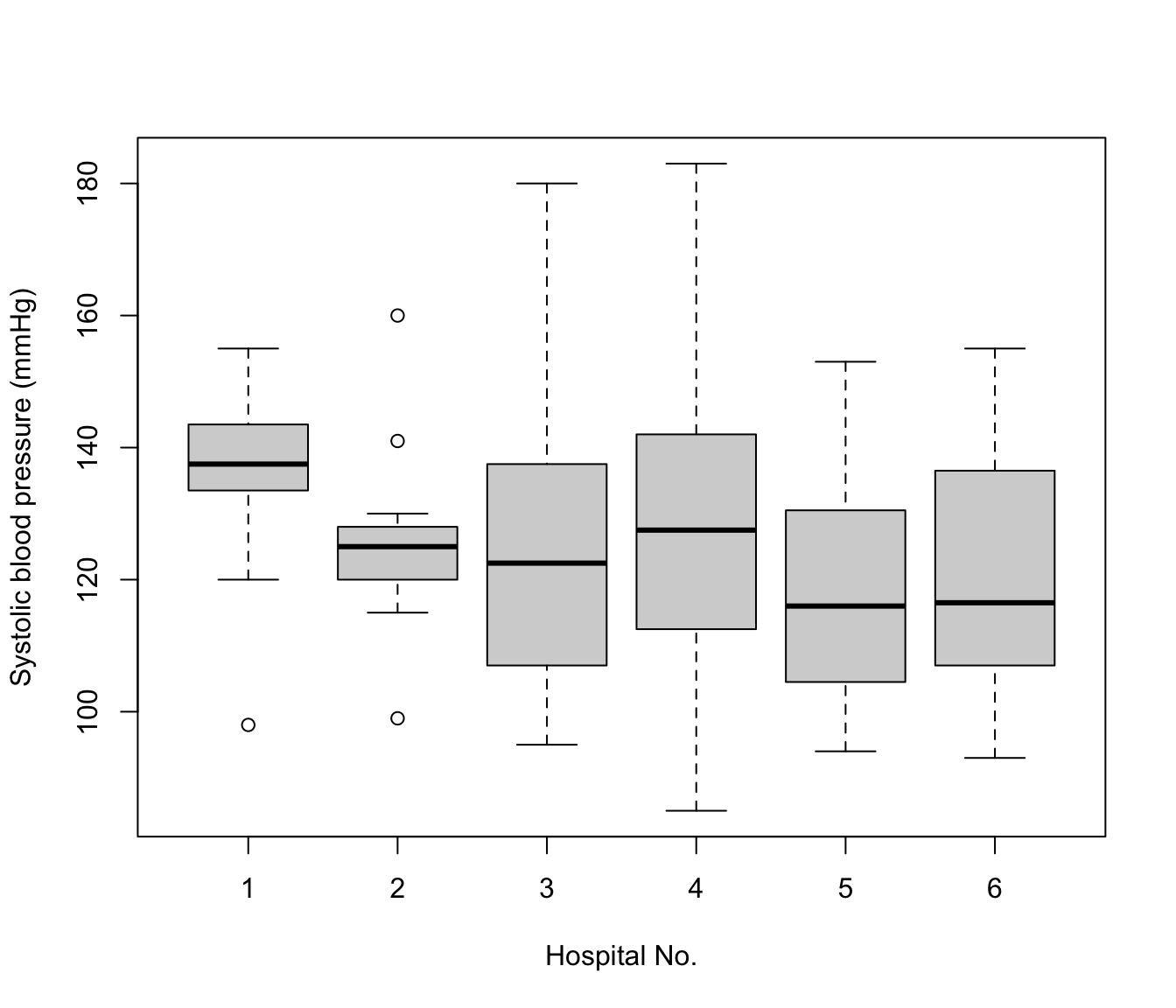
圖 72.1: Box and whiskers plot of measured SBP in patients from six hospitals
- 圖 72.2 展示的是對 17 名患者使用兩種不同的測量方法測量的最大呼吸速率 (peak-expiratory-flow rate, PEFR)。兩種方法又測量了兩次,途中展示的是其中一種測量方法前後兩次測量結果的散點圖。
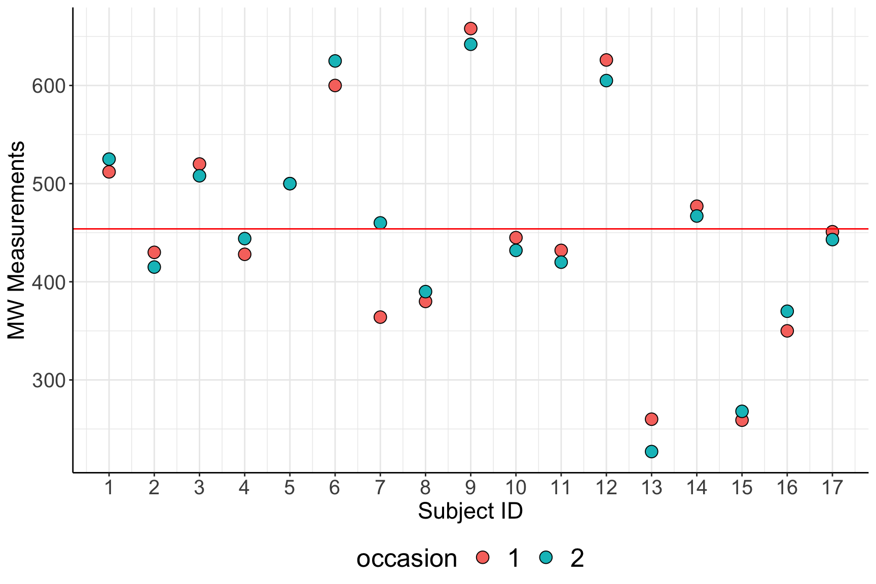
圖 72.2: Two recordings of PEFR taken with the Mini Wright meter
- 圖 72.3 展示的來自全英 65 所學校的 4059 名學生入學前閱讀水平測試成績 (LRT) 和畢業時 GCSE 考試成績之間的散點圖關系。值得注意的是該圖其實無視了學校這個變量,把每個學生看成相互獨立的個體。但是當我們隨機選取四所學校,看它們各自的學生的成績表現 (圖 72.4)。很顯然,之前忽視了學校這一層級的變量是不恰當的,因爲不同學校學生的入學前和畢業時成績之間的相關性很明顯存在不同的模式 (四所學校的回歸線各自的截距和斜率各不相同)。
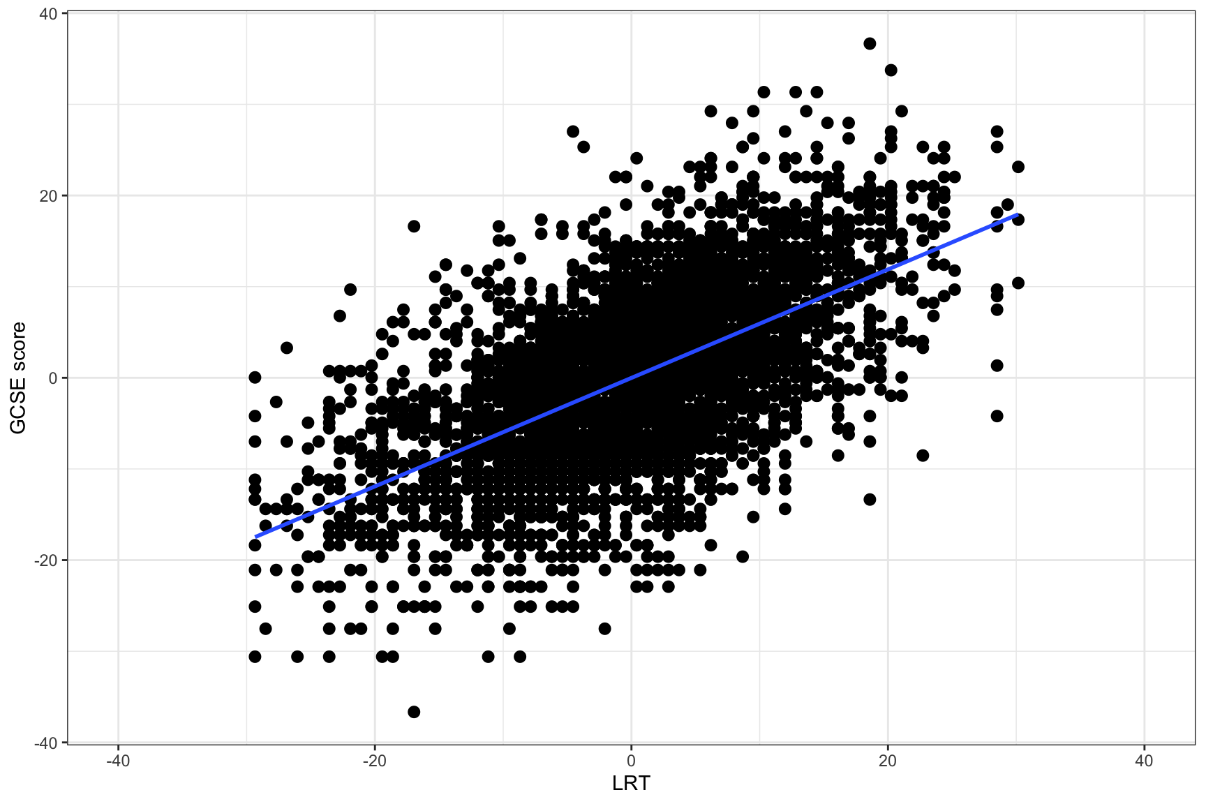
圖 72.3: GCSE by LRT in all 65 schools
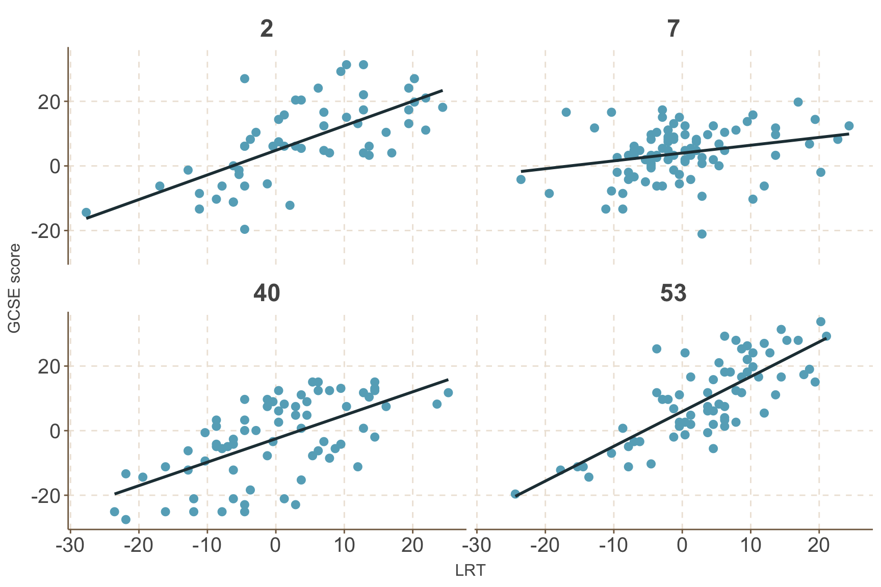
圖 72.4: GCSE by LRT in four randomly selected schools
- 另一個特別好的例子展示在圖 72.5 中,是關於同一個母親的不同孩子的出生體重的數據。一個母親可以有多個孩子,每個母親的孩子之間的出生體重很明顯無法看作相互獨立。圖中展示的是,3300 名生了兩個孩子的母親的孩子們出生體重的散點圖。同一個母親的小孩用線相連。顯然,同一個母親生的孩子,其出生體重比不同母親的孩子出生體重差距更小,更接近彼此,因爲他們來自同一個母親。可以想象,一個母親如果身材高大,那麼她的孩子們可能都傾向於有比較高的出生體重。所以同一個母親的孩子之間體重是有相關關系的 (within correlation)。
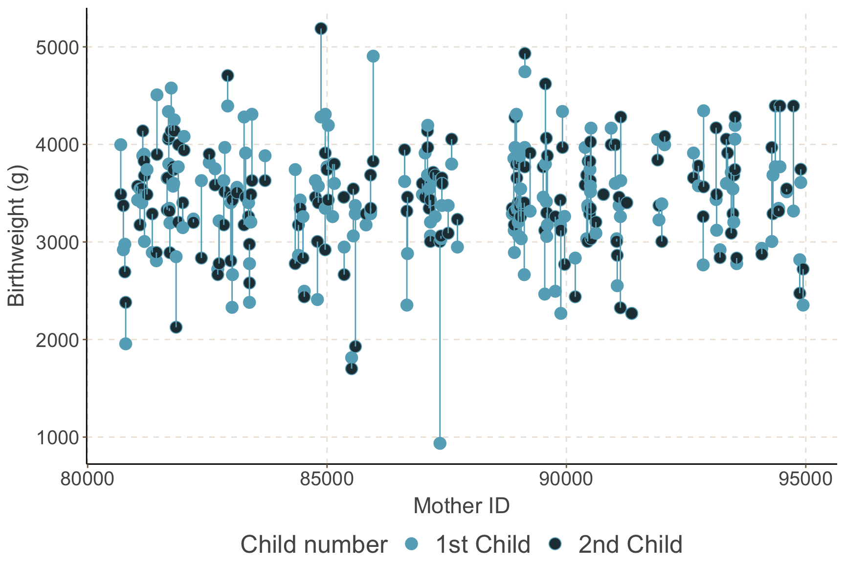
圖 72.5: Birthweight of siblings by maternal identifier
- 最後一個用於本章節的實例是,一項研究亞洲兒童生長狀況的調查分別記錄了 198 個數據點,68 個兒童在 0 到 3 歲之間的四個年齡點的體重數據。圖 72.6 展示的就是這個典型的隨訪數據的個人生長曲線。且圖中每個人的生長軌跡提示,男孩子的生長過程可能相互之間體重差異顯得較女孩子來得大。如果,我們用每個兒童自己的數據,給每個兒童擬合各自的回歸線,數據顯然不足,但是如果我們決定忽略個體的生長的隨機效應 (不均一性),又顯得十分不妥當。
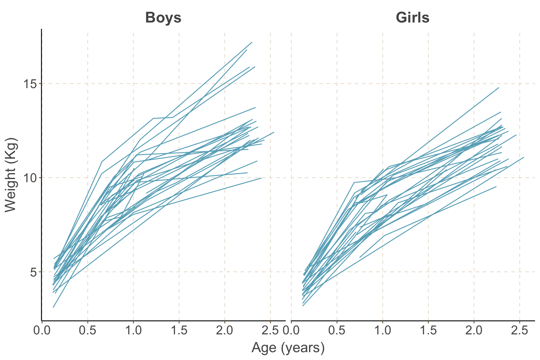
圖 72.6: Growth profiles of boys and girls in the Asian growth data
72.2 依賴性的來源在哪裏
上述例子中的數據,均提示我們數據與數據之間獨立性的假設,常常會遇到尷尬的局面。因爲數據與數據之間本身就不可能完全獨立。
- 同一個診所或者醫院的患者,他們之間可能有着某些相似的因素從而導致他們的血壓相比其他醫院的人彼此更加接近。這個原因可能是有同一家醫院的患者可能有類似的疾病。
- 同一患者身上反復抽取樣本,也就是說一個對象貢獻了多個數據的時候,這些來自同一對象的數據當然具有相對不同對象數據更高的均質性。
- 同一所學校的學生的成績或內部的相關性,很可能大於不同學校兩個學生之間成績的相關性。因爲同一學校的孩子可能共享某些共同的特徵,比如說相似的家庭經濟背景,或者是同樣的教學內容教學老師等環境因素。這樣,來自同一所學校的孩子的成績很可能就會更加相似。
- 至於說家庭數據就更加典型了。來自同一家庭的兄弟姐妹,有着極強的相關性,因爲他們共享着遺傳因素,或者是相似的家庭教育/飲食/生活習慣等環境因素。
- 同一個體身上的縱向 (時間) 隨訪數據很顯然會比不同患者有更強的內部相關性。
目前位置介紹的這些常見實例中,可以發現它們有一個共通點。就是這些數據其實內部是有分層結構的 (hierarchy)。這些數據中,都有一個最底層單元 (elementary units/level 1),還有一個聚合單元 (aggregate units/level 2),聚合單元常被命名爲層級 (cluster)。
| Aggregate | Elementary |
|---|---|
| hospitals | patients |
| individuals | PEFR measures |
| schools | pupils |
| mothers | children |
| children | visits |
正如表格 72.1 總結的那樣,這些數據中存在這層級結構,這種數據被稱爲分層數據 (hierarchical),或者叫嵌套式數據 (nested data)。根據你所在的知識領域,它可能還被命名爲多層結構數據 (multilevel and clustered data)。在一些研究中,你可能會遇見從實驗設計階段就存在分層結構的數據,比如使用分層抽樣 (multistage sampling) 的設計的實驗等。這樣的實驗設計最常在人口學,社會學的研究中看到。在大多數醫學研究中,每個數據點 (observation point, level 1),所屬的層 (cluster) 本身可能是我們感興趣的研究點 (例如同屬於一個家庭,相同母親的後代),又或者是同一個人/患者的隨着時間推移的隨訪健康狀態 (如生長曲線,體重變化,疾病康復情況)。
如果用前面用過的 圖 72.6 的生長曲線做例子,那麼每個被調查的兒童,就是該數據的第二級層,每個隨訪時刻測量的體重數據,則是觀察的數據點。這個數據還有一個特點是,觀察數據點是有前後的 (時間) 順序的,這是一個典型的縱向研究數據 (longitudinal data)。
72.3 數據有依賴性導致的結果
如果你手頭的數據,結構上是一種嵌套式結構數據,那麼任何無視了這一點作出的統計學推斷都是有瑕疵的。相互之間互不獨立這一特質,需要通過一種新的手段,把嵌套式的數據結構考慮進統計學模型裏來。
在一些情況下,數據的嵌套式結構可能可以被忽略掉,但是其結果是導致統計學的估計變得十分低效 (inefficient procedure)。你可能會聽說過一般化估計公式 (generalized estimating equations),是其中一種備擇手段,因爲在這一公式中,你需要人爲地指定數據與數據之間可能的依賴關系是怎樣的。
其實,即使有人真的在分析過程中忽略了數據本身的嵌套式結構,他會發現最終在描述分析結果的時候,還是無法避免這一嚴重的問題。另外一些統計學家可能記得在穩健統計學法中,三明治標準誤估計法也是可以供選擇的一種處理相關數據的手段。
72.4 邊際模型和條件模型 marginal and conditional models
邊際模型和條件模型的概念其實不是分層模型特有的,卻在分析分層數據模型時十分有用。假如,對於某個結果變量 \(Y\) 有它如下的回歸模型,其中我們把某個單一的共變量 \(Z\) 從模型中分離出來,加以特別關注:
\[ g\{ \text{E}(Y|\textbf{X},Z) \} = \beta\textbf{X} +\gamma Z \]
這是一個典型的條件模型,它描述了結果變量 \(Y\) 的期望是以怎樣的條件和解釋變量 \(\textbf{X},Z\) 之間建立關系的。每個解釋變量的回歸系數,其含義都是以其他同一模型中的共變量不變的條件下,和結果變量之間的關系。經過這樣的解讀,你會知道,其實本統計學教程目前爲止遇見過的所有的回歸模型都是條件模型。如果此時我們反過來思考,把上述模型中單獨分離出來的單一共變量 \(Z\) 對於結果變量 \(Y\) 均值的影響合並起來 (對共變量 \(Z\) 積分即可),此時我們得到的就是共變量 \(\textbf{X}\) 和結果變量 \(Y\) 之間,關於 \(Z\) 的邊際模型 (Marginal model):
\[ \text{E}_Z\{ \text{E}(Y|\textbf{X}, Z) \} = \text{E}_Z\{ g^{-1}(\beta\textbf{X} + \gamma Z) \} \\ \text{Where } \text{E}(Z) = 0 \]
用線性回歸來舉例:
\[ \text{E}(Y| \textbf{X}, Z) = \beta\textbf{X} + \gamma Z \]
那麼此時共變量 \(\textbf{X}\) 的邊際模型回歸系數 \(\beta\) 的含義,和條件模型時的回歸系數其實是相同的含義:
\[ \text{E}_Z\{\text{E}(Y|\textbf{X},Z)\} = \text{E}_Z(\beta\textbf{X} + \gamma Z) = \beta\textbf{X} + \gamma\text{E}(Z) = \beta\textbf{X} \]
爲什麼這裏的邊際模型對於分層數據來說很重要呢?答案在於,嵌套式數據中,我們常常關心那第二個階層 (重復測量某個指標的患者,學生成績數據中的學校層級,等) 在它所在的那個階層中和結果變量之間的平均關系。(In models for hierarchical data we often use level effects to represent what is common among observations from one “cluster” or “group”. We may then want marginal conclusions: we need to average over these effects).
72.4.1 標記法 notation
- \(Y_{ij}\) 標記第 \(j\) 層的第 \(i\) 個個體;
- \(i = 1, \cdots, n_j\) 表示第 \(j\) 層中共有 \(n_j\) 個個體 (elements);
- \(j = 1, \cdots, J\) 表示數據共有 \(J\) 個第二階層 (clusters);
- \(N = \sum_{j=1}^J n_j\) 表示總體樣本量等於各個階層樣本量之和;
- 特殊情況: 如果每個階層的個體數相同 \(n\),\(N=nJ\),這樣的數據被叫做均衡數據 (balanced data)。
72.4.2 合並每個階層
過去常見的總結嵌套式數據的手段只是把每層數據取平均值,這樣的方法簡單粗暴但是偶爾是可以接受的,只要你能夠接受如此處理數據可能帶來的如下後果:
- 各層數據均值,其可靠程度 (方差) 隨着各層的樣本量不同而不同 (depends on the number of elementary units per cluster);
- 變量的含義發生改變。如果是使用層水平 (cluster level) 的數據,本來測量給個體的那些變量,就變成了層的變量,從此作出的任何統計學推斷,只能限制在層水平 (ecological fallacy, as correlations at the macro level cannot be used to make assertions at the micro level);
- 由於無視了層內個體數據,導致大量信息損失。
此處我們借用 (Snijders and Bosker 1999) 書中第 28 頁的人造數據,如下表
| Cluster \((j)\) | id \((i)\) | \(X\) | \(Y\) | \(\bar{X}\) | \(\bar{Y}\) |
|---|---|---|---|---|---|
| 1 | 1 | 1 | 5 | 2 | 6 |
| 1 | 2 | 3 | 7 | 2 | 6 |
| 2 | 1 | 2 | 4 | 3 | 5 |
| 2 | 2 | 4 | 6 | 3 | 5 |
| 3 | 1 | 3 | 3 | 4 | 4 |
| 3 | 2 | 5 | 5 | 4 | 4 |
| 4 | 1 | 4 | 2 | 5 | 3 |
| 4 | 2 | 6 | 4 | 5 | 3 |
| 5 | 1 | 5 | 1 | 6 | 2 |
| 5 | 2 | 7 | 3 | 6 | 2 |
這個表中的人造數據,其結構是一目了然的,它的第二層級數量是 5,每層的個體數量是 2。這是一個平衡數據。由於這是個我們人爲模擬的數據,圖 72.7 也顯示它沒有隨機誤差,所有數據都在各自的直線上。
dt <- read.csv("../backupfiles/hierexample.csv", header = T)
names(dt) <- c("Cluster", "id", "X", "Y", "Xbar", "Ybar")
dt$Cluster <- as.factor(dt$Cluster)
ggthemr('fresh')

ggplot(dt, aes(x = X, y = Y, shape = Cluster, colour = Cluster)) + geom_point(size =5) +
  theme(axis.text = element_text(size = 15),
  axis.text.x = element_text(size = 15),
  axis.text.y = element_text(size = 15)) +
  labs(x = "X", y = "Y")  +
  theme(axis.title = element_text(size = 17), axis.text = element_text(size = 8)) +
theme(legend.position = "bottom", legend.direction = "horizontal") + theme(legend.text = element_text(size = 19), legend.title = element_text(size = 19))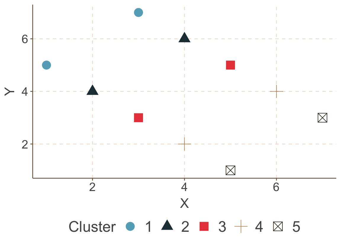
圖 72.7: Artificial data: scatter of clustered data
- 如果我們無視其分層數據的嵌套式結構,把每個數據都看作是獨立的樣本,擬合一個整體回歸 (total regression) 圖 72.8:
\[ \hat Y_{ij} = 5.33 - 0.33 X_{ij} \]
ggthemr('fresh')

ggplot(dt, aes(x = X, y = Y)) + geom_point(size = 5, shape = 23) +
  geom_smooth(method = "lm", se = FALSE, linetype = 2) +
  theme(axis.text = element_text(size = 15),
  axis.text.x = element_text(size = 15),
  axis.text.y = element_text(size = 15)) +
  labs(x = "X", y = "Y")  +
  theme(axis.title = element_text(size = 17), axis.text = element_text(size = 8)) +
theme(legend.position = "bottom", legend.direction = "horizontal") + theme(legend.text = element_text(size = 19), legend.title = element_text(size = 19))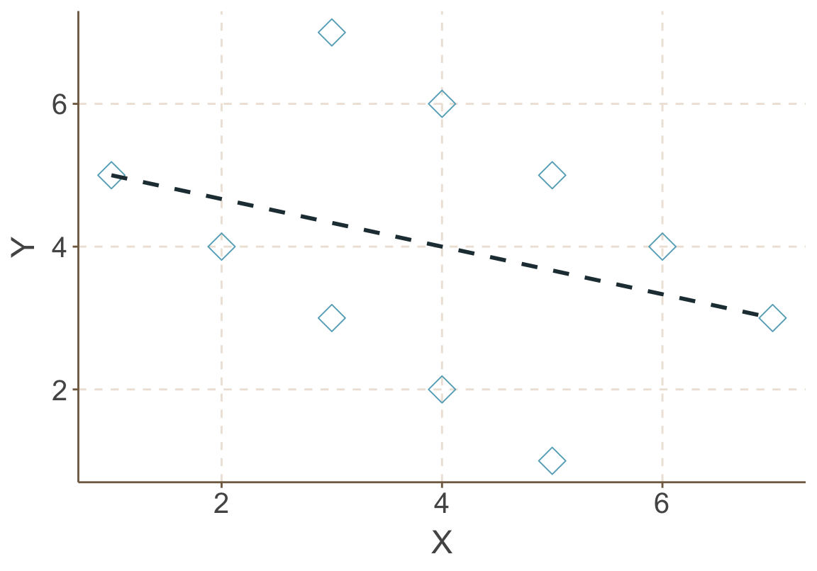
圖 72.8: Artificial data: Total regression
- 如果我們只保留層級數據本身,求了變量 \(X,Y\) 在每層的均值的話,就得到了層間回歸 (between regression) 圖 72.9 – 變量 \(X,Y\) 之間的回歸直線的斜率變得更大了:
\[ \hat{\bar{Y}}_j = 8.0 - 1.0 \bar{X}_j \]
ggthemr('fresh')

ggplot(dt, aes(x = X, y = Y)) + geom_point(size =5, shape=23) +
    geom_smooth(method = "lm", se = FALSE, linetype = 2) +
  geom_abline(intercept = 8, slope = -1) +
  geom_point(aes(x = Xbar, y=Ybar, size = 5)) +
  theme(axis.text = element_text(size = 15),
  axis.text.x = element_text(size = 15),
  axis.text.y = element_text(size = 15)) +
  labs(x = "X", y = "Y")  +
  theme(axis.title = element_text(size = 17), axis.text = element_text(size = 8)) + theme(legend.position="none")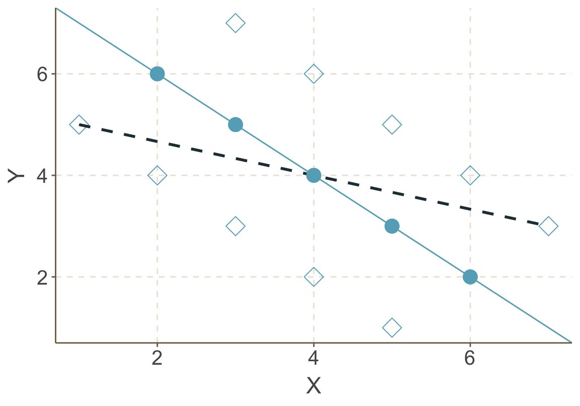
圖 72.9: Artificial data: scatter of clustered data
72.4.3 生物學悖論 ecological fallacy
生物學悖論常見於我們認爲某分層數據中層級變量之間的關系,同樣適用與層級中的個體之間: 例如比較 A 國 和 B 國之間心血管疾病的發病率,發現 A 國國民食鹽平均攝入量高於 B 國,很多人可能就會下結論說食鹽攝入量高的個體,心血管疾病發病的危險度較高。然而,這樣的推論很多時候是錯誤的。
曾經在 (W. S. Robinson 1950) 論文中舉過的著名例子: 該研究調查美國每個州的移民比例,和該州相應的識字率之間的關系。研究者發現,移民比例較高的州,其識字率也較高 (相關系數 0.53)。由此就有人下結論說移民越多,那個州的教育水平會比較高。但是實際情況是,把每個個體的受教育水平和該個體本身是不是移民做了相關系數分析之後發現,這個關系其實是負相關 (-0.11)。所以說在州的水平作出的統計學推斷-移民多的州受教育水平高-是不正確的。之所以在州水平發現移民比例和受教育水平之間的正關系,是因爲移民傾向於居住在教育水平本來就比較高的本土出生美國人的州。
72.4.4 分解層級數據
如果是分析最初層級數據 (level 1) 的話,我們還需要考慮下列一些問題:
- 當心數據被多次利用
如果我們關心的變量其實是在第二層級的 (level 2/cluster level),但是你卻把它當作是第一層級的數據,就會引起數據很多的錯覺,因爲同一層的個體他們的層屬變量都是一樣的,你擁有的數據其實並沒有你想的那麼多。
前文中用過的 GCSE 數據其實是一個很好的例子,下表中歸納了調查的學校類型 (男校,女校或者混合校),以及按照每個學生個人所屬學校類型的總結,可以看出,當你嘗試使用個人 (elementary level) 水平的數據分析實際上是第二層級數據的特性時,你會被誤導。因爲個人數據告訴你, 34% 的學生在女校學習,然而正確的分析法應該是,學校中有 31% 的學校是女校。
| N | % | N | % | |
|---|---|---|---|---|
| mixed | 35 | 54 | 2169 | 53 |
| boys only | 10 | 15 | 513 | 13 |
| girls only | 20 | 31 | 1377 | 34 |
| Total | 65 | 100 | 4059 | 100 |
- 分層數據分析法
有人會說,既然如此,那麼我們就把數據放在每層當中分析就好了 (stratified analyses)。還是用前文中用過的人造 5 層數據來說明這樣做的弊端。前面用了兩種方法 (total regression, between regression) 來總結這個 5 層的人造數據 72.9。最後一種分析此數據的方法是,把 5 層數據分開分別做回歸線如圖 72.10。等同於我們的對數據擬合五次下面的回歸方程:
\[ \hat Y_{ij} - \bar{Y}_j = \beta(X_{ij} - \bar{X}_j) \]
這種模型被叫做層內回歸 (within regression)。這 5 個線性回歸的斜率都是 1,是五條不同截距的平行直線。因爲我們自己編造的數據的緣故,現實數據不太可能恰好所有層內回歸的斜率都是完全相同的。這其實也是曾內回歸法的一個默認前提 – 每層數據中解釋變量和結果變量之間的關系是相同的。
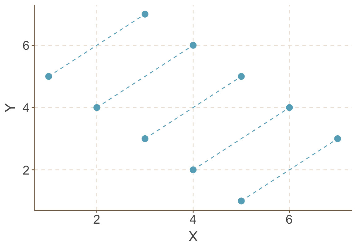
圖 72.10: Artificial data: within cluster regressions
72.4.5 固定效應模型 fixed effect model
無論數據中的分層結構是否有現實意義 (如果說是五種不同的民族,那就有顯著的現實意義),在回歸模型中都有必要考慮這個分層結構對數據的變異的貢獻 (the contribution of the clusters to the data variation)。
線性回歸章節中我們使用的是五個啞變量來代表不同組別加以分析:
\[ Y_{ij} = \alpha_1 I_{i, j = 1} + \alpha_2 I_{i, j=2} + \cdots + \alpha_5 I_{i, j=5} + \beta_1X_{ij} + \varepsilon_{ij} \]
其中 \(j\) 是所屬層級編號。該模型中的 \(\varepsilon_{ij}\) 被認爲服從均值爲零,方差爲 \(\sigma_{\varepsilon}^2\) 的正態分布。該模型也可以簡寫爲:
\[ Y_{ij} = \alpha_j + \beta_1X_{ij} + \epsilon_{ij} \] 一樣一預案 這樣的模型在等級線性回歸模型中被認爲是固定效應模型 fixed effect model。它其實是默認給五個層級五個不同的截距,每層內部 \(X,Y\) 之間的關系 (斜率) 則被認爲是完全相同的 (namely the within cluster models are the same)。
本課剛開始的例子中有個數據是來自 6 所不同醫院 72 名患者的收縮期血壓的數據。我們現在來分析這些人中血壓和年齡之間的關系。下面的散點圖重現了六所醫院的72名患者的血壓和年齡。
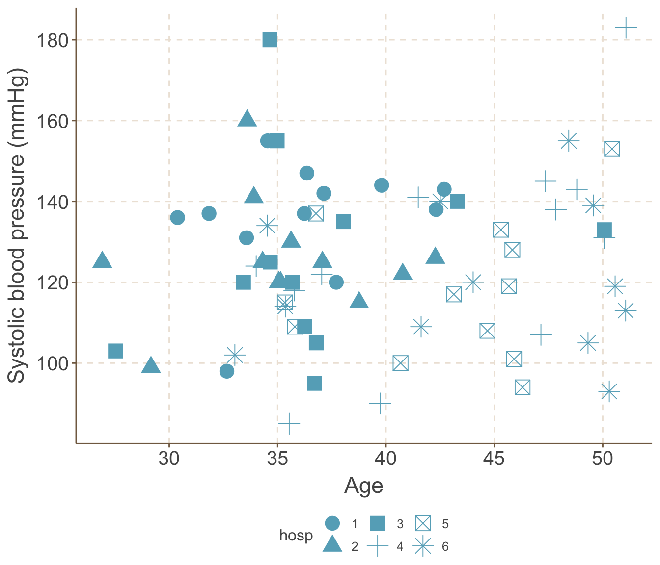
圖 72.11: SBP versus age: different symbols identify the six hospitals
下面在 R 裏擬合這個固定效應模型:
Bp <- read_dta("../backupfiles/bp.dta")

Bp$hosp <- as.factor(Bp$hosp)
Bp <- Bp %>%
  mutate(c_age = age - mean(age))
# 通過指定截距爲零,獲取每個醫院的回歸線的截距
Model0 <- lm(bp ~ 0 +  c_age + hosp, data = Bp)

summary(Model0)
##
## Call:
## lm(formula = bp ~ 0 + c_age + hosp, data = Bp)
##
## Residuals:
## Min 1Q Median 3Q Max
## -34.7803 -9.8106 -0.5285 7.4000 55.5287
##
## Coefficients:
## Estimate Std. Error t value Pr(>|t|)
## c_age 1.00223 0.43766 2.290 0.02528 *
## hosp1 139.15421 5.73015 24.285 < 2e-16 ***
## hosp2 130.21017 5.86957 22.184 < 2e-16 ***
## hosp3 129.58146 5.66881 22.859 < 2e-16 ***
## hosp4 124.00188 5.70326 21.742 < 2e-16 ***
## hosp5 114.58859 5.70289 20.093 < 2e-16 ***
## hosp6 115.79702 5.85632 19.773 < 2e-16 ***
## ---
## Signif. codes: 0 '***' 0.001 '**' 0.01 '*' 0.05 '.' 0.1 ' ' 1
##
## Residual standard error: 19.136 on 65 degrees of freedom
## Multiple R-squared: 0.97954, Adjusted R-squared: 0.97733
## F-statistic: 444.46 on 7 and 65 DF, p-value: < 2.22e-16# 先生成一個新的醫院變量 hops1 = 1。然後使用偏 F 檢驗法
# 檢驗控制了患者的年齡以後,這六所醫院的截距是否各自不相同。
Bp$hosp1 <- Bp$hosp[1]
mod2 <- lm(bp ~ 0 + c_age + as.numeric(hosp1), data = Bp)
anova(Model0, mod2)## Analysis of Variance Table
##
## Model 1: bp ~ 0 + c_age + hosp
## Model 2: bp ~ 0 + c_age + as.numeric(hosp1)
## Res.Df RSS Df Sum of Sq F Pr(>F)
## 1 65 23801.9
## 2 70 27751.6 -5 -3949.73 2.15725 0.069638 .
## ---
## Signif. codes: 0 '***' 0.001 '**' 0.01 '*' 0.05 '.' 0.1 ' ' 1偏 F 檢驗法給出的結果 \(F(5, 65) = 2.16, P = 0.07\),所以說,數據其實告訴我們,調整了年齡之後,這六所醫院患者中年齡和血壓之間關系的回歸線有不同的截距。
72.5 簡單線性迴歸複習
滾回線性回歸章節 27。
72.6 Practical Hierarchical 01
72.6.1 數據
- High-School-and-Beyond 數據
本數據來自1982年美國國家教育統計中心 (National Center for Education Statistics, NCES) 對美國公立學校和天主教會學校的一項普查。曾經在 Hierarchical Linear Model (Raudenbush and Bryk 2002) 一書中作爲範例使用。其數據的變量名和各自含義如下:
minority           indicatory of student ethinicity (1 = minority, 0 = other)
female             pupil's gender
ses                standardized socio-economic status score
mathach            measure of mathematics achievement
size               school's total number of pupils
sector             school's sector: 1 = catholic, 0 = not catholic
schoolid school identifier- PEFR 數據
數據本身是 17 名研究對象用兩種不同的測量方法測量兩次每個人的最大呼氣流速 (peak-expiratory-flow rate, PEFR)。最早在1986年的柳葉刀雜誌發表 (Bland and Altman 1986)。兩種測量法的名稱分別是 “Standard Wright” 和 “Mini Wright” peak flow meter。變量名和個字含義如下:
id                 participant identifier
wp1                standard wright measure at 1st occasion
wp2                standard wright measure at 2nd occasion
wm1                mini wright measure at 1st occasion
wm2 mini wright measure at 2nd occasion72.6.3 將 High-School-and-Beyond 數據導入 R 中,熟悉數據結構及內容,特別要注意觀察每個學校的學生特徵。
hsb_selected <- read_dta("../backupfiles/hsb_selected.dta")
length(unique(hsb_selected$schoolid)) ## number of school = 160
## [1] 160## create a subset data with only the first observation of each school
hsb <- hsb_selected[!duplicated(hsb_selected$schoolid), ]
## about 44 % of the schools are Catholic schools
with(hsb, tab1(sector, graph = FALSE, decimal = 2))## sector :
## Frequency Percent Cum. percent
## 0 90 56.25 56.25
## 1 70 43.75 100.00
## Total 160 100.00 100.00## among all the pupils, about 53% are females
with(hsb_selected, tab1(female, graph = FALSE, decimal = 2))## female :
## Frequency Percent Cum. percent
## 0 3390 47.18 47.18
## 1 3795 52.82 100.00
## Total 7185 100.00 100.00## among all the pupils, about 27.5% are from ethnic minorities
with(hsb_selected, tab1(minority, graph = FALSE, decimal = 2))## minority :
## Frequency Percent Cum. percent
## 0 5211 72.53 72.53
## 1 1974 27.47 100.00
## Total 7185 100.00 100.0072.6.4 爲了簡便起見,接下來的分析只節選數據中前五所學校 188 名學生的數學成績,和 SES。分別計算每所學校的數學成績,及 SES 的平均值。
hsb5 <- subset(hsb_selected, schoolid < 1320)
Mean_ses_math <- ddply(hsb5,~schoolid,summarise,mean_ses=mean(ses),mean_math=mean(mathach))
## the mean SES score ranges from -0.4255 to +0.5280
## the mean Maths score ranges from 7.636 to 16.255
Mean_ses_math
## schoolid mean_ses mean_math
## 1 1224 -0.43438298 9.7154468
## 2 1288 0.12159999 13.5108000
## 3 1296 -0.42550000 7.6359583
## 4 1308 0.52800000 16.2554999
## 5 1317 0.34533333 13.177687572.6.5 先無視掉學校這一分層變量,把所有學生看作是相互獨立的,擬合總體的 SES 和數學成績的線性迴歸 (Total regression model)。把該總體模型的預測值提取並存儲在數據庫中。
## plot the scatter of mathach and ses among these 5 schools

ggplot(hsb5, aes(x = ses, y = mathach)) + geom_point() +
  theme_bw() +
  theme(axis.text = element_text(size = 15),
  axis.text.x = element_text(size = 15),
  axis.text.y = element_text(size = 15)) +
  labs(x = "SES", y = "Math achievement")  +
  xlim(-2.05, 2.05)+
  ylim(-10, 30) +
  theme(axis.title = element_text(size = 17), axis.text = element_text(size = 8))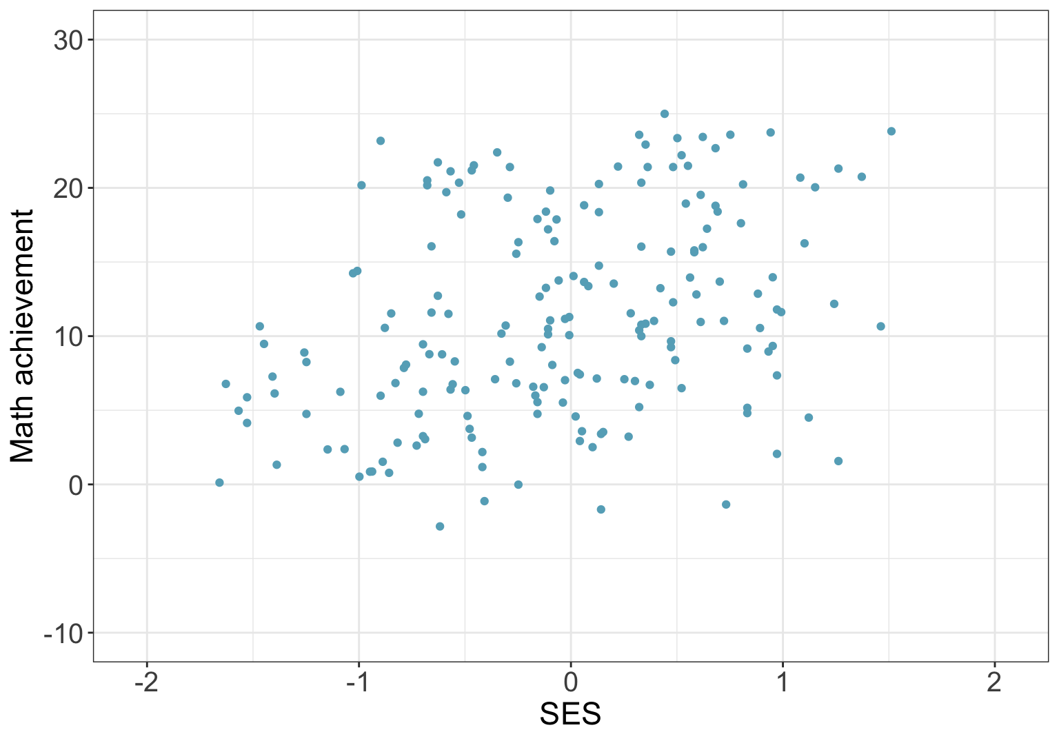
圖 72.12: Scatter plot of SES and math achievements among all pupils from first 5 schools, assuming that they are all independent
Total_reg <- lm(mathach ~ ses, data = hsb5)
## the total regression model gives an estimated regression coefficient for the SES
## of each pupil equal to 3.31 (SE=0.66)
summary(Total_reg)
##
## Call:
## lm(formula = mathach ~ ses, data = hsb5)
##
## Residuals:
## Min 1Q Median 3Q Max
## -15.23022 -5.08316 -0.68614 5.11170 14.68513
##
## Coefficients:
## Estimate Std. Error t value Pr(>|t|)
## (Intercept) 11.45652 0.47342 24.1997 < 2.2e-16 ***
## ses 3.30696 0.66021 5.0089 1.267e-06 ***
## ---
## Signif. codes: 0 '***' 0.001 '**' 0.01 '*' 0.05 '.' 0.1 ' ' 1
##
## Residual standard error: 6.4708 on 186 degrees of freedom
## Multiple R-squared: 0.11886, Adjusted R-squared: 0.11412
## F-statistic: 25.09 on 1 and 186 DF, p-value: 1.2667e-0672.6.6 用各個學校 SES 和數學成績的均值擬合一個學校間的線性迴歸模型 (between regression model)。
Btw_reg <- lm(mean_math ~ mean_ses, data = Mean_ses_math)
## the regression model for the school level variables (between model) gives
## an estimated regression coefficient of 7.29 (SE=1.41)
summary(Btw_reg)
##
## Call:
## lm(formula = mean_math ~ mean_ses, data = Mean_ses_math)
##
## Residuals:
## 1 2 3 4 5
## 1.02010 0.76212 -1.12415 0.54401 -1.20209
##
## Coefficients:
## Estimate Std. Error t value Pr(>|t|)
## (Intercept) 11.86216 0.55664 21.3102 0.0002261 ***
## mean_ses 7.29039 1.40703 5.1814 0.0139557 *
## ---
## Signif. codes: 0 '***' 0.001 '**' 0.01 '*' 0.05 '.' 0.1 ' ' 1
##
## Residual standard error: 1.2418 on 3 degrees of freedom
## Multiple R-squared: 0.89949, Adjusted R-squared: 0.86598
## F-statistic: 26.847 on 1 and 3 DF, p-value: 0.01395672.6.7 分別對每個學校內的學生進行 SES 和數學成績擬合線性迴歸模型。
Within_schl1 <- lm(mathach ~ ses, data = hsb5[hsb5$schoolid == 1224,])
Within_schl2 <- lm(mathach ~ ses, data = hsb5[hsb5$schoolid == 1288,])
Within_schl3 <- lm(mathach ~ ses, data = hsb5[hsb5$schoolid == 1296,])
Within_schl4 <- lm(mathach ~ ses, data = hsb5[hsb5$schoolid == 1308,])
Within_schl5 <- lm(mathach ~ ses, data = hsb5[hsb5$schoolid == 1317,])
# the within school regressions gives estimated slopes which have a mean of 1.65
# and which ranges between 0.126 and 3.255
summary(c(Within_schl1$coefficients[2], Within_schl2$coefficients[2],
      Within_schl3$coefficients[2], Within_schl4$coefficients[2],
      Within_schl5$coefficients[2]))
## Min. 1st Qu. Median Mean 3rd Qu. Max.
## 0.12602 1.07596 1.27391 1.64799 2.50858 3.25545# the SEs ranging between 1.21 and 3.00
summary(c(summary(Within_schl1)$coefficients[4],
summary(Within_schl2)$coefficients[4],
summary(Within_schl3)$coefficients[4],
summary(Within_schl4)$coefficients[4],
summary(Within_schl5)$coefficients[4]))## Min. 1st Qu. Median Mean 3rd Qu. Max.
## 1.2090 1.4359 1.7652 1.8987 2.0797 3.003472.6.8 比較三種模型計算的數學成績的擬合值,他們一致?還是有所不同?爲什麼會有不同?
- 總體模型 (Total regression model) 實際上無視了學生的性別,種族等可能帶來的混雜效果;
- 學校間模型 (Between model) 估計的實際上是SES均值每增加一個單位,與之對應的數學平均成績的改變量,這個模型絕對不可用與評估個人的 SES 與數學成績之間的關係;
- 學校內模型 (Within model) 擬合的 SES 與數學成績之間的關係變得十分地不精確 (SEs are fairly large),變化幅度也很大。
72.6.9 把三種模型的數學成績擬合值散點圖繪製在同一張圖內。
Mean <- Mean_ses_math[, 1:3]
names(Mean) <- c("schoolid", "ses", "Pred_W")


ggplot(hsb5, aes(x = ses, y = Pred_W, group = schoolid)) +
  geom_line(linetype = 2, size = 1) +
  geom_abline(intercept = Total_reg$coefficients[1], slope = Total_reg$coefficients[2],
               colour = "dark blue") +
  geom_abline(intercept = Btw_reg$coefficients[1], slope = Btw_reg$coefficients[2],
               colour = "red") +
  geom_point(data = Mean, shape = 17, size = 4, colour = "Red") +
  theme_bw() +
  theme(axis.text = element_text(size = 15),
  axis.text.x = element_text(size = 15),
  axis.text.y = element_text(size = 15)) +
  labs(x = "SES", y = "Fitted regression lines (Maths achievement)")  +
  xlim(-2.05, 2.05)+
  ylim(5, 20) +
  theme(axis.title = element_text(size = 17), axis.text = element_text(size = 8)) +
  theme(plot.caption = element_text(size = 12,
  hjust = 0)) + labs(caption = "Black dash line: Within regression model;
Blue solid line: Total regression model;
Red solid line: Between regression model;
Red triangle: School mean values")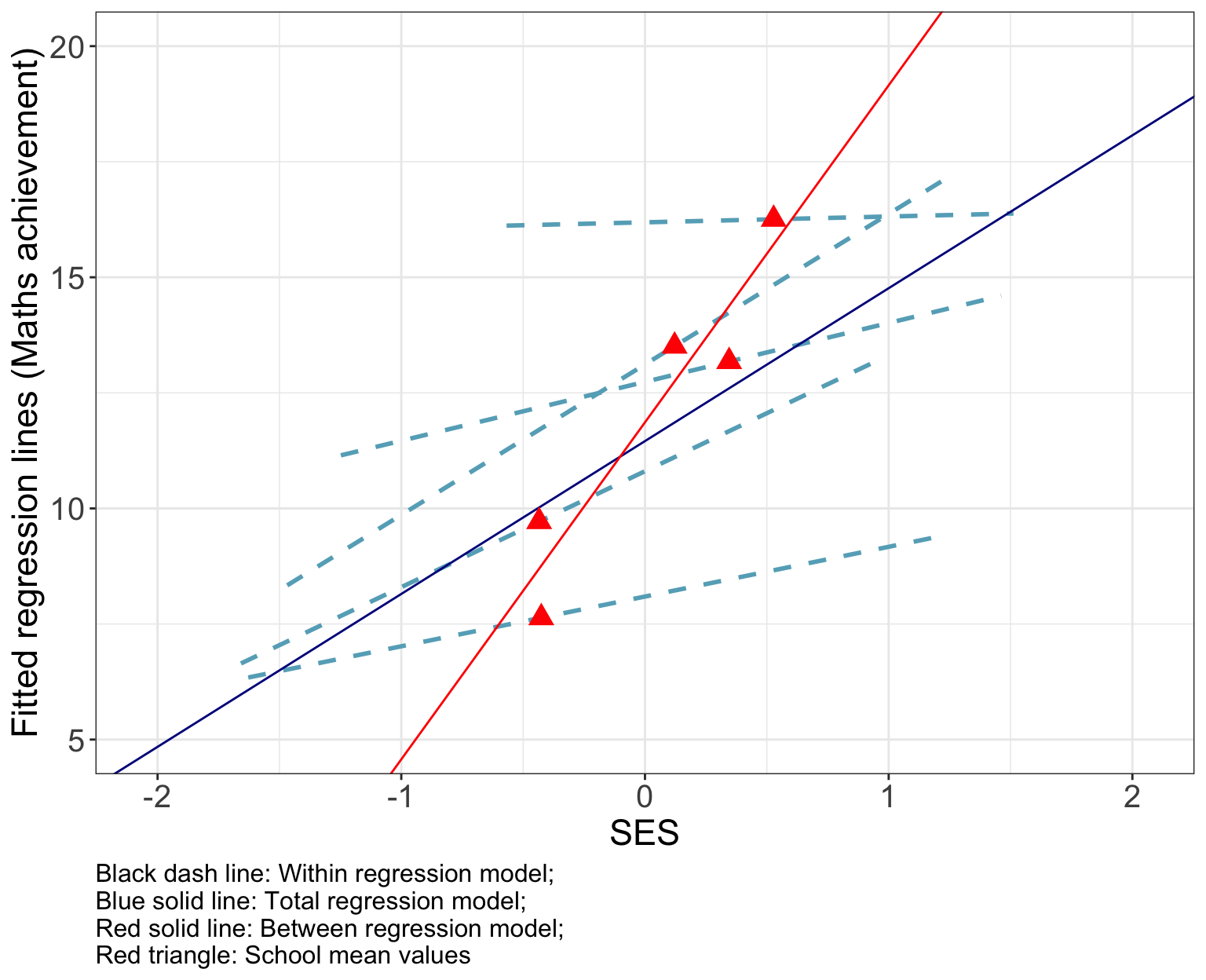
圖 72.13: High-school-and-beyond data: Predicted values by Total, Between, and Within regression models
72.6.10 用這 5 個學校的數據擬合一個固定效應線性迴歸模型
Fixed_reg <- lm(mathach ~ ses + factor(schoolid), data = hsb5)

## Fitting a fixed effect model to these data is equivalent to forcing
## a common slope onto the five within regression models. It gives an
## estimated slope of 1.789 (SE=0.76), close to their average of 1.64799.
## Note that controlling for female, minority, and sector but not for
## schoolid leads to roughly the same estimate (slope = 1.68, SE=0.75)

summary(Fixed_reg)
##
## Call:
## lm(formula = mathach ~ ses + factor(schoolid), data = hsb5)
##
## Residuals:
## Min 1Q Median 3Q Max
## -13.97593 -4.19683 -0.75189 5.22088 16.38133
##
## Coefficients:
## Estimate Std. Error t value Pr(>|t|)
## (Intercept) 10.49254 0.96761 10.8438 < 2.2e-16 ***
## ses 1.78896 0.75939 2.3558 0.019548 *
## factor(schoolid)1288 2.80072 1.60041 1.7500 0.081803 .
## factor(schoolid)1296 -2.09538 1.27973 -1.6374 0.103283
## factor(schoolid)1308 4.81839 1.81826 2.6500 0.008758 **
## factor(schoolid)1317 2.06736 1.41005 1.4662 0.144332
## ---
## Signif. codes: 0 '***' 0.001 '**' 0.01 '*' 0.05 '.' 0.1 ' ' 1
##
## Residual standard error: 6.2362 on 182 degrees of freedom
## Multiple R-squared: 0.1992, Adjusted R-squared: 0.1772
## F-statistic: 9.0544 on 5 and 182 DF, p-value: 1.0512e-07##
## Call:
## lm(formula = mathach ~ ses + female + minority + sector, data = hsb5)
##
## Residuals:
## Min 1Q Median 3Q Max
## -13.09128 -4.17332 -0.46306 4.50807 15.33205
##
## Coefficients:
## Estimate Std. Error t value Pr(>|t|)
## (Intercept) 12.54543 0.86027 14.5831 < 2.2e-16 ***
## ses 1.68055 0.74489 2.2561 0.0252480 *
## female -1.54861 0.94857 -1.6326 0.1042780
## minority -3.19635 0.95450 -3.3487 0.0009857 ***
## sector 3.98121 1.11941 3.5565 0.0004785 ***
## ---
## Signif. codes: 0 '***' 0.001 '**' 0.01 '*' 0.05 '.' 0.1 ' ' 1
##
## Residual standard error: 6.1696 on 183 degrees of freedom
## Multiple R-squared: 0.2119, Adjusted R-squared: 0.19467
## F-statistic: 12.301 on 4 and 183 DF, p-value: 7.0265e-0972.6.11 讀入 PEFR 數據。
## # A tibble: 17 × 5
##       id   wp1   wp2   wm1   wm2
##    <dbl> <dbl> <dbl> <dbl> <dbl>
##  1     1   494   490   512   525
##  2     2   395   397   430   415
##  3     3   516   512   520   508
##  4     4   434   401   428   444
##  5     5   476   470   500   500
##  6     6   557   611   600   625
##  7     7   413   415   364   460
##  8     8   442   431   380   390
##  9     9   650   638   658   642
## 10    10   433   429   445   432
## 11    11   417   420   432   420
## 12    12   656   633   626   605
## 13    13   267   275   260   227
## 14    14   478   492   477   467
## 15    15   178   165   259   268
## 16    16   423   372   350   370
## 17    17   427   421   451   443
# transform data into long format
pefr_long <- pefr %>%
gather(key, value, -id) %>%
separate(key, into = c("measurement", "occasion"), sep = 2) %>%
arrange(id, occasion) %>%
spread(measurement, value)
pefr_long## # A tibble: 34 × 4
## id occasion wm wp
## <dbl> <chr> <dbl> <dbl>
## 1 1 1 512 494
## 2 1 2 525 490
## 3 2 1 430 395
## 4 2 2 415 397
## 5 3 1 520 516
## 6 3 2 508 512
## 7 4 1 428 434
## 8 4 2 444 401
## 9 5 1 500 476
## 10 5 2 500 470
## # … with 24 more rows## figure shows slightly closer agreement between the repeated measures of standard Wright,
## than between those of Mini Wright
ggplot(pefr_long, aes(x = id, y = wp, fill = occasion)) +
geom_point(size = 4, shape = 21) +
geom_hline(yintercept = mean(pefr_long$wp), colour = "red") +
theme_bw() +
scale_x_continuous(breaks = 1:17)+
theme(axis.text = element_text(size = 15),
axis.text.x = element_text(size = 15),
axis.text.y = element_text(size = 15)) +
labs(x = "Subject ID", y = "W Measurements") +
theme(axis.title = element_text(size = 17), axis.text = element_text(size = 8))+
theme(legend.text = element_text(size = 19),
legend.title = element_text(size = 19))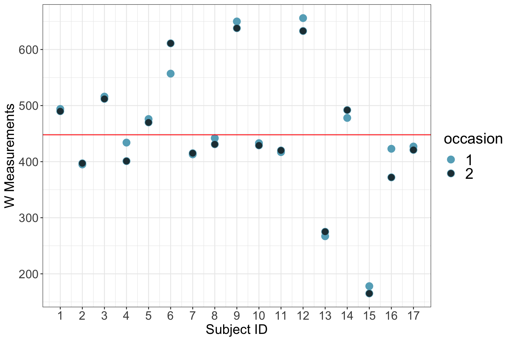
圖 72.14: Two recordings of PEFR taken with the standard Wright meter
72.6.12 求每個患者的 wp 兩次測量平均值
## # A tibble: 17 × 2
##       id mean_wp
##    <dbl>   <dbl>
##  1     1    492
##  2     2    396
##  3     3    514
##  4     4    418.
##  5     5    473
##  6     6    584
##  7     7    414
##  8     8    436.
##  9     9    644
## 10    10    431
## 11    11    418.
## 12    12    644.
## 13    13    271
## 14    14    485
## 15    15    172.
## 16    16    398.
## 17    17    424
72.6.13 在 R 裏先用 ANOVA 分析個人的 wp 變異。再用 lme4::lmer 擬合用 id 作隨機效應的混合效應模型。確認後者報告的 Std.Dev for id effect 其實可以用 ANOVA 結果的 \(\sqrt{\frac{\text{MMS-MSE}}{n}}\) (n 是每個個體重複測量值的個數)。
## Analysis of Variance Table
##
## Response: wp
##            Df Sum Sq  Mean Sq F value    Pr(>F)
## factor(id) 16 441599 27599.91   117.8 3.145e-14 ***
## Residuals  17   3983   234.29
## ---
## Signif. codes: 0 '***' 0.001 '**' 0.01 '*' 0.05 '.' 0.1 ' ' 1## Linear mixed model fit by REML ['lmerModLmerTest']
## Formula: wp ~ (1 | id)
## Data: pefr_long
## REML criterion at convergence: 353.5472
## Random effects:
## Groups Name Std.Dev.
## id (Intercept) 116.974
## Residual 15.307
## Number of obs: 34, groups: id, 17
## Fixed Effects:
## (Intercept)
## 447.88## [1] 116.9743672.6.14 擬合結果變量爲 wp,解釋變量爲 id 的簡單線性迴歸模型。用數學表達式描述這個模型。
Reg <- lm(wp ~ factor(id), data = pefr_long)

# The fixed effect regression model leads to the same ANOVA
# table. To the same estimate of the residual SD = (15.307)
# However, it does not give an estimate of the "SD of id effect"
# Instead it gives estimates of mean PEFR for participant number 1
# = 492 and estimates of the difference in means from him/her
# for all the other 16 pariticipants
anova(Reg)
## Analysis of Variance Table
##
## Response: wp
## Df Sum Sq Mean Sq F value Pr(>F)
## factor(id) 16 441599 27599.91 117.8 3.145e-14 ***
## Residuals 17 3983 234.29
## ---
## Signif. codes: 0 '***' 0.001 '**' 0.01 '*' 0.05 '.' 0.1 ' ' 1##
## Call:
## lm(formula = wp ~ factor(id), data = pefr_long)
##
## Residuals:
## Min 1Q Median 3Q Max
## -27.00 -3.75 0.00 3.75 27.00
##
## Coefficients:
## Estimate Std. Error t value Pr(>|t|)
## (Intercept) 492.000 10.823 45.4569 < 2.2e-16 ***
## factor(id)2 -96.000 15.307 -6.2718 8.435e-06 ***
## factor(id)3 22.000 15.307 1.4373 0.1687894
## factor(id)4 -74.500 15.307 -4.8672 0.0001448 ***
## factor(id)5 -19.000 15.307 -1.2413 0.2313547
## factor(id)6 92.000 15.307 6.0105 1.405e-05 ***
## factor(id)7 -78.000 15.307 -5.0958 8.972e-05 ***
## factor(id)8 -55.500 15.307 -3.6259 0.0020883 **
## factor(id)9 152.000 15.307 9.9303 1.715e-08 ***
## factor(id)10 -61.000 15.307 -3.9852 0.0009574 ***
## factor(id)11 -73.500 15.307 -4.8018 0.0001662 ***
## factor(id)12 152.500 15.307 9.9630 1.635e-08 ***
## factor(id)13 -221.000 15.307 -14.4382 5.665e-11 ***
## factor(id)14 -7.000 15.307 -0.4573 0.6532334
## factor(id)15 -320.500 15.307 -20.9386 1.413e-13 ***
## factor(id)16 -94.500 15.307 -6.1738 1.020e-05 ***
## factor(id)17 -68.000 15.307 -4.4425 0.0003571 ***
## ---
## Signif. codes: 0 '***' 0.001 '**' 0.01 '*' 0.05 '.' 0.1 ' ' 1
##
## Residual standard error: 15.307 on 17 degrees of freedom
## Multiple R-squared: 0.99106, Adjusted R-squared: 0.98265
## F-statistic: 117.8 on 16 and 17 DF, p-value: 3.145e-14上面的模型用數學表達式來描述就是:
\[ \begin{aligned} Y_{ij} & = \alpha_1 + \delta_i + \varepsilon_{ij} \\ \text{Where } \delta_j & = \alpha_j - \alpha_1 \\ \text{and } \delta_1 & = 0 \end{aligned} \]
72.6.15 將 wp 中心化之後,重新擬合相同的模型,把截距去除掉。寫下這個模型的數學表達式。
Reg1 <- lm((wp - mean(wp)) ~ 0 + factor(id), data = pefr_long)

# it leads to the same ANOVA table again, same residual SD
anova(Reg1)
## Analysis of Variance Table
##
## Response: (wp - mean(wp))
## Df Sum Sq Mean Sq F value Pr(>F)
## factor(id) 17 441599 25976.38 110.871 4.5349e-14 ***
## Residuals 17 3983 234.29
## ---
## Signif. codes: 0 '***' 0.001 '**' 0.01 '*' 0.05 '.' 0.1 ' ' 1##
## Call:
## lm(formula = (wp - mean(wp)) ~ 0 + factor(id), data = pefr_long)
##
## Residuals:
## Min 1Q Median 3Q Max
## -27.00 -3.75 0.00 3.75 27.00
##
## Coefficients:
## Estimate Std. Error t value Pr(>|t|)
## factor(id)1 44.118 10.823 4.0761 0.0007863 ***
## factor(id)2 -51.882 10.823 -4.7935 0.0001692 ***
## factor(id)3 66.118 10.823 6.1087 1.158e-05 ***
## factor(id)4 -30.382 10.823 -2.8071 0.0121232 *
## factor(id)5 25.118 10.823 2.3207 0.0329951 *
## factor(id)6 136.118 10.823 12.5762 4.894e-10 ***
## factor(id)7 -33.882 10.823 -3.1305 0.0060933 **
## factor(id)8 -11.382 10.823 -1.0516 0.3076854
## factor(id)9 196.118 10.823 18.1197 1.493e-12 ***
## factor(id)10 -16.882 10.823 -1.5598 0.1372300
## factor(id)11 -29.382 10.823 -2.7147 0.0147164 *
## factor(id)12 196.618 10.823 18.1659 1.432e-12 ***
## factor(id)13 -176.882 10.823 -16.3425 7.887e-12 ***
## factor(id)14 37.118 10.823 3.4294 0.0031978 **
## factor(id)15 -276.382 10.823 -25.5355 5.342e-15 ***
## factor(id)16 -50.382 10.823 -4.6549 0.0002269 ***
## factor(id)17 -23.882 10.823 -2.2065 0.0413886 *
## ---
## Signif. codes: 0 '***' 0.001 '**' 0.01 '*' 0.05 '.' 0.1 ' ' 1
##
## Residual standard error: 15.307 on 17 degrees of freedom
## Multiple R-squared: 0.99106, Adjusted R-squared: 0.98212
## F-statistic: 110.87 on 17 and 17 DF, p-value: 4.5349e-14上面的模型用數學表達式來描述就是:
\[ \begin{aligned} Y_{ij} - \mu & = \gamma_j + \varepsilon_{ij} \\ Y_{ij} & = \mu + \gamma_j + \varepsilon_{ij} \\ \text{Where } \mu & \text{ is the overall mean} \\ \text{and } \sum_{j=1}^J\gamma_j & = 0\\ \end{aligned} \]
72.6.16 計算這些迴歸係數 (其實是不同羣之間的隨機截距) 的均值和標準差。
# the individual level intercepts have mean zero and SD = 117.47, larger than the estimated
# Std.Dev for id effect.
Reg1$coefficients
## factor(id)1 factor(id)2 factor(id)3 factor(id)4 factor(id)5 factor(id)6 factor(id)7
## 44.117647 -51.882353 66.117647 -30.382353 25.117647 136.117647 -33.882353
## factor(id)8 factor(id)9 factor(id)10 factor(id)11 factor(id)12 factor(id)13 factor(id)14
## -11.382353 196.117647 -16.882353 -29.382353 196.617647 -176.882353 37.117647
## factor(id)15 factor(id)16 factor(id)17
## -276.382353 -50.382353 -23.882353## [1] 1.4628821e-14## [1] 117.47321