第 101 章 貝葉斯廣義線性回歸

第五章(Chapter 99.1)中我們已經展示過如何在貝葉斯統計學語境下如何描述和運算簡單線性回歸模型的過程：

• 描述預測變量和結果變量之間應有的關係；
• 描述結果變量的概率分佈假設 (probability assumptions)：也就是在前一步指定的方程式描述的預測變量和相應的參數的條件下，結果變量的分佈。
• 給每個回歸係數，以及其他未知的參數提供先驗概率分佈的信息。

對於一個結果變量 \(y_i\) 來說，如果有一個預測變量的向量 \(x_1, \dots, x_p\)，來描述它 \(i = 1,\dots, n\) 個個體的話，標準的貝葉斯版本的線性回歸模型要寫作：

\[ \begin{aligned} y_i & \sim N(\mu_i, \sigma^2) \\ \mu_i & = \beta_0 + \sum_{i = 1}^p\beta_jx_{ji} \\ (\beta_0, \beta_1, \dots, \beta_p) & \sim \text{ Prior distributions } \\ \end{aligned} \tag{101.1} \]

用貝葉斯方法建立回歸模型的優點有很多。首先，你可以方便地對未知的回歸係數等參數加入相關的先驗概率分佈用來表達已有的知識，或者對回歸係數加以合理的限制。其次，你可以從容地對回歸模型的擬合效果，預測能力做出統計學推斷。再加上，使用貝葉斯方法也很容易讓我們把模型擴展到非線性回歸模型，處理並分析缺失值，以及分析共變量的測量誤差等等。

更重要的是，MCMC方法讓我們人類也可以很容易地進行穩健的統計推斷 (robust inference)。例如上面的線性回歸模型中，如果有理由認為誤差服從的是自由度為4的 t 分佈，那就可以把第一行模型似然改寫成為：

\[ y_i \sim t_4(\mu_i, \sigma^2) \]

使用t分佈作為模型似然的話，相比高斯模型(正態分佈)可以調低(downweight)離群值(outliers)的權重。(詳見 Chapter 99.2.9)

實際上，貝葉斯廣義線性回歸模型(Bayesian GLM)直觀地可以被認為是貝葉斯線性回歸模型的擴展模型。記得在基礎的廣義線性回歸模型章節，我們學習過如何用一個鏈接方程(link function)把結果變量(outcome)，和解釋變量用數學表達式連接起來。廣義線性回歸模型中最常見的莫過於邏輯回歸模型，接下來我們就來看看如何在貝葉斯統計學框架下擬合我們想要的邏輯回歸模型。在這之前，我們先要學習如何在BUGS語言下描述一個分類型變量(categorical variable)。

101.1 如何在BUGS語言中描述分類型變量

雖然 BUGS 語言風格和 R 語言十分接近，但是二者並不完全通用。BUGS並無像R語言一樣有Factor因子型變量的概念來表述分類型數據。相似的概念在BUGS語言中可以有兩種方法來表達：

• 人工把分類型變量編輯成為啞變量的方式，然後把啞變量輸入數據框中；
• 利用BUGS語言方便的索引功能 (indexing facilities)。

下面我們用簡單線性回歸模型來解釋這兩種方法的異同，其中一個分類型解釋變量 \(x_i\)，它有 \(A,B,C\) 三種分型(例如ABO血型只有三種分類時的情況)，其中 A 是三個分類中的參照組(reference group)。

101.1.1 啞變量的數據矩陣

用啞變量矩陣的方式表達分類型變量是常用的手段，為一個有三個分類的變量生成啞變量我們需要給出兩個指示變量(indicator variable)，其中 \(x2=1\) 時表示 \(x_i = B\)，\(x2=0\)時表示 \(x_i\neq B\)，\(x3=1\) 時表示\(x_i = C\)，\(x3=0\) 時表示 \(x_i\neq C\)：

y[]    x2[]    x3[]
32     0       0        # x_i=A
21     0       0
...
6      0       0
15     1       0        # x_i=B
24     1       0     
...
12     1       0
7      0       1        # x_i=C
26     0       1
...
19     0       1
END

此時，這個模型的BUGS表達式可以寫作：

for (i in 1:n) {
      y[i]  ~ dnorm(mu[i], tau) 
      mu[i] <- alpha + beta2*x2[i] + beta3*x3[i]
}

alpha ~ dunif(-1000, 1000)
beta2 ~ dunif(-1000, 1000)
beta3 ~ dunif(-1000, 1000)
tau   ~ dgamma(0.001, 0.001)

其中，

• alpha 是參照組 \(x_i = A\) 的結果變量的均值；
• beta2 是和參照組相比，\(x_i = B\) 的結果變量的均值和參照組之間結果變量均值的差；
• beta3 是和參照組相比，\(x_i = C\) 的結果變量的均值和參照組之間結果變量均值的差。

101.1.2 雙重索引BUGS語言標記法

與前面的啞變量矩陣描述相異的，我們可以利用BUGS語言中便捷的索引方法來描述一個分類型變量，例如用 \(x = 1\) 表示 \(x_i = A\)，用 \(x = 2\) 表示 \(x_i = B\)，用 \(x = 3\) 表示 \(x_i = C\)：

y[]      x[]
32       1               # x = A
21       1 
... 
6        1
15       2               # x = B
24       2 
...
12       2
7        3               # x = C
26       3
...
19       3
END

此時，相同的模型則需要被表達成爲：

for(i in 1:n) {
    y[i] ~ dnorm(m[i], tau)
    mu[i] <- alpha + beta[x[i]]
}
alpha ~ dunif(-1000, 1000)
beta[1] <- 0   # fixed as baseline class
beta[2] ~ dunif(-1000, 1000)
beta[3] ~ dunif(-1000, 1000)
tau ~ dgamma(0.001, 0.001)

可以注意到我們在這個模型中把參考組的回歸系數篤定在了 0。這時候，我們給起始值數據時，就不需要給 beta[1] 指定起始值了：

list(alpha = 10, beta = c(NA, -2, 4), tau = 1)

101.2 邏輯回歸 Bayesian Logistic Regression

對於一個二分類的結果變量 (binary outcome variable) 來說，最自然的模型是使用邏輯回歸模型。

假如每個個體都有一個二分類結果變量 \(y_i = 0 \text{ or } 1\)。那麼每個個體 \(i\) 的結果 \(y_i\) 可以用伯努利分布 (Chapter 4) 來描述它：

\[ y_i \sim Bern(p_i) \]

其中，\(p_i\)是第\(i\)個個體的結果變量取1時\((y_i = 1)\)的概率。此時 \(P(p_i = 1)\) 是我們想要知道的需要用貝葉斯模型來擬合的未知參數。邏輯回歸模型中我們使用的鏈接方程是 \(\mathbf{logit}\)：

\[ \theta_i = \text{logit}(p_i) = \log(\frac{p_i}{1-p_i}) \]

\(\mathbf{logit}\)鏈接方程允許我們把一個只能在 \((0,1)\) 之間取值的概率數據，映射到可以在 \((-\infty, +\infty)\) 之間取值的變量，之後我們再把這個變量和預測變量使用線性方程連接起來：

\[ \text{logit}(p_i) = \alpha + \sum_k\beta_kx_{ki} \tag{101.2} \]

這個模型的似然方程，它的事後概率分布是無法獲得閉合解的 (closed form)，但是但是，MCMC強大的計算機模擬過程幫我們解決了這個棘手的問題。

###　邏輯回歸模型中回歸系數的含義

在表達式 (101.2) 中我們可以對每個回歸系數做出如下的定義：

• \(\alpha\) 是當所有的預測變量取值同時爲零時的結果變量的對數比值 (log odds)：

\[ \Rightarrow \text{logit}^{-1}(\alpha) = \frac{e^\alpha}{(1+e^\alpha)} = \text{ probability of the outcome when all covariates are set to zero} \]

• \(\beta_k\) 則是預測變量 \(x_k\) 發生一個單位變化時，引起的結果變量的變化的對數比值比 (log odds ratio)：

\[ \Rightarrow e^{\beta_k} = \text{ odds ratio of outcome per unit change in } x_k \]

101.2.1 低出生體重數據

本例子中，我們關心的研究問題是，三氯甲烷 (trihalomethane, THM)濃度和生下的新生兒爲低出生體重之間是否相關。THM已知是使用氟化氫(chlorine)對飲用水消毒時可能產生副產品，被認爲可能對人類生殖系統造成一定的傷害。數據收集到931名新生兒體重數據，該數據包含的變量有：

• lbw 是該新生兒出生時體重是否爲低體重的二分類變量。
• thm 是一個指示變量，當它爲0時表示暴露的THM爲低水平，當它爲1時表示暴露的THM爲高水平。
• age 是一個關於母親們年齡的分類型變量 (1 = $$25歲，2 = 25-29歲，3 = 30-34 歲，4 = \(\geqslant\) 35歲)。
• male 表示新生兒的性別 (0 是女孩，1 是男孩)。
• car 是一個表示貧困程度的指數。
• smoke 是表示母親在懷孕期間是否有吸煙習慣的變量 (0 = 無吸煙習慣，1 = 有吸煙習慣)。

要回答我們關心的研究問題，那麼這個數據中，

• lbw 是結果變量；
• thm 是暴露變量；
• age, male, car, smoke 是可能影響暴露變量和結果之間關係的混雜因子 (confounders)。

這時候，本例中的貝葉斯模型的數學表達式可以寫作：

\[ \begin{aligned} lbw_i & \sim Bernoulli(p_i) \;\; [\text{equivalent to } Binomial(p_i, 1)] \\ \text{logit}(p_i) & = \alpha + \beta_{thm}thm_i + \beta^T_C\mathbf{C}_i \\ \alpha, \beta_{thm}, \dots & \sim \text{Normal}(0, 10000^2) \\ e^{\beta_{thm}}& = \text{odds ratio of low birth weight for high v low thm exposure} \end{aligned} \]

其中 \(\mathbf{C}\) 是混雜因子組成的向量。也就是母親的年齡，新生兒的性別，貧困指數，以及母親孕期吸煙史。

利用OpenBUGS的雙重索引功能來標記分類型變量的話，這個低體重數據可以被整理為：

lbw[] thm[] age[] male[] car[] smoke[]
0     0     1     1      0.156   1
0     0     3     0     -2.165   1
0     1     1     0     -1.391   1
1     1     4     0      0.156   1
......
0     1     3     1      0.930   0
END

其對應的BUGS模型代碼為：

model{
    ### MODEL ###
    for (i in 1:931) { # loop through 931 individuals
       y[i] ~ dbern(p[i])
       logit(p[i]) <-  alpha+beta.thm*thm[i]+beta.age[age[i]]+beta.male*male[i]+
       beta.car*car[i]+beta.smoke*smoke[i]
    }
    ### PRIORS ###
    alpha ~ dnorm(0,0.00000001)
    beta.thm ~ dnorm(0,0.00000001)
    beta.age[1] ~ dnorm(0,0.00000001)
    beta.age[2] <- 0 # alias second level of maternal age beta
    beta.age[3] ~ dnorm(0,0.00000001)
    beta.age[4] ~ dnorm(0,0.00000001)
    beta.male ~ dnorm(0,0.00000001)
    beta.car ~ dnorm(0,0.00000001)
    beta.smoke ~ dnorm(0,0.00000001)
    ### CALCULATE THE ODDS RATIOS ###
    OR.thm <- exp(beta.thm)
    OR.age1 <- exp(beta.age[1])
}

OpenBUGS中刨除前5000次樣本採集之後，獲取30000個位置參數的事後樣本，我們獲得了如下的結果：

         mean   sd     MC_error val2.5pc median val97.5pc
beta.thm 0.7587 0.4181 0.008799 -0.02731 0.7453 1.631
OR.thm   2.337  1.074  0.02403  0.9731   2.107  5.107

所以，我們獲得事後比值比2.337的含義就是，孕期暴露高劑量THM和低劑量的THM相比，新生兒出生體重為低出生體重的比值是2.3 (95% 可信區間 credible intervals: 0.97, 5.11)。

值得注意的是，我們上面獲得的事後beta.thm均值，並不等於OR.thm均值取對數：\(0.7587 \neq log(2.337)\)。

101.3 貝葉斯泊鬆回歸 Bayesian Poisson Regression

泊鬆回歸用於對計數型數據做回歸模型，例如死亡人數，住院人數，發病人數等。對計數型結果變量使用泊鬆模型時，我們對發生事件的次數的均值的對數加以數學模型：\(\mu_i = E(y_i)\)

\[ \begin{aligned} y_i & \sim Poi(\mu_i) \\ \log (\mu_i) & = \alpha + \sum_k\beta_kx_{ki} \end{aligned} \]

泊鬆模型的數學公式同時也暗示我們默認結果事件發生次數的均值，取對數以後和解釋變量之間呈線性關系。同樣地，高斯先驗概率分布(正態分布)長用於這樣廣義線性回歸模型中的未知參數。

101.4 GLM in a Bayesian way

• 各種你學過的廣義線性回歸模型均可以使用貝葉斯統計學的方法來描述並分析，通過MCMC獲得模型中每個未知參數的事後概率分布描述。
• 各種你學過的廣義線性回歸模型使用的標準鏈接方程，都可以照搬過來用在貝葉斯廣義線性會回歸模型中。
• 因爲我們用 MCMC 方法對各個未知參數的事後概率分布進行樣本採集，我們有極其靈活的先驗概率分布描述手段。回歸系數的先驗概率分布通常可以使用高斯分布(正態分布)，一般來說會設定均值爲0，方差合適的正態分布作爲先驗概率分布。
• 使用貝葉斯統計學框架，廣義線性回歸模型的右邊，可以被擴展至任何非線性回歸模型。強大的計算機模擬過程幫我們解決了無法獲得閉合解這一大難題。

101.5 Practical Bayesian Statistics 07

要點：

• 學會用OpenBUGS跑貝葉斯邏輯回歸模型；
• 懂得如何解讀，解釋貝葉斯廣義線性回歸模型結果中的參數估計；
• 使用DIC比較不同的貝葉斯模型。

數據來自研究 (Diggle et al. 2002)，該研究設計是爲了評價 National Impregnated Bednet Programme 是否能減少岡比亞兒童瘧疾發病率，及由於瘧疾導致的死亡。當時研究者從2035名岡比亞兒童身上採集了血樣，用於化驗是否有瘧原蟲感染。同時收集的變量包括，兒童的年齡，兒童是否有規律地使用蚊帳，以及使用的蚊帳是否是經過 (permethrin insecticide) 殺蟲。另外還收集的兩個村莊水平 (village level) 的變量分別是，兒童生活的村莊是否受 Primary Health Care System 管轄，以及村莊環境中的植被情況 (greenness of the village environment)。

該試驗數據除了對使用蚊帳和罹患瘧疾之間的關係進行評估之外，還希望能通過收集到的數據分析是否存在超二項變異 (extra-binomial variation)的證據。這裏，超二項變異的含義是，在調整了已測量的全部觀察變量以後，仍然存在其他未知或者是未測量的潛在因子，導致殘留的差異(residual differences)無法被解釋。

原始數據是個人級別的 (1 record per child)。這裏爲了練習的需要，我們對數據進行了整理彙總，這樣的數據其實使用 MCMC 採集事後樣本效率也比較高。且我們的練習題用的數據只是研究地區西部25個村莊構成的局部數據。這樣，經過處理後的數據庫保存有805名兒童的數據，他們的彙總後的數據有149個二項變量 (binomial categories)。

數據保存在 malaria-data.txt 文件中，使用的是方形格式 (rectangular format)，它有如下的幾個變量:

POP[] MALARIA[] AGE[] BEDNET[] GREEN[] PHC[] VILLAGE[] 
3     2         2     1        40.85   1      1
1     1         3     1        40.85   1      1
2     2         4     1        40.85   1      1
7     3         1     2        40.85   1      1
5     1         2     2        40.85   1      1
6     3         3     2        40.85   1      1
... 
END

• POP 是所有變量組合下兒童的人數；
• MALARIA 是所有變量組合下兒童感染虐原蟲兒童的人數；
• AGE 表示年齡分組 (1 = 0-2 歲，2 = 2-3 歲，3 = 3-4 歲，4 = 4-5 歲)；
• BEDNET 表示使用蚊帳的情況分類 (1 = 不使用蚊帳，2 = 使用未經殺蟲劑處理過的蚊帳，3 = 使用經過殺蟲劑處理過的蚊帳)；
• GREEN 是表示村莊植被環境的一個連續型指標；
• PHC 是一個二分類數據，1/0 = 該村莊是/不是受到 Primary Health Care System 管轄。
• VILLAGE 是村莊的代碼。

1. 使用貝葉斯邏輯迴歸模型估計使用蚊帳與否和虐原蟲感染之間的關係。嘗試寫下這個貝葉斯模型的BUGS表達文件，並且注意計算:

• 參照組(也就是未使用蚊帳組)兒童的瘧疾感染率 (百分比)
• 每一個可能的共變量的比值比
• 使用蚊帳和不使用蚊帳相比，能夠降低兒童患瘧疾的比值(odds)的概率；
  使用殺蟲劑處理過的蚊帳和使用未處理過的蚊帳相比，能夠降低兒童患瘧疾的比值的概率；
  

模型可以寫作:

# Logistic regression model for malaria data
    
model {
   for(i in 1:149) {
      MALARIA[i] ~ dbin(p[i], POP[i])
      logit(p[i]) <- alpha + beta.age[AGE[i]] + beta.bednet[BEDNET[i]] +
                                   beta.green*(GREEN[i] - mean(GREEN[])) + beta.phc*PHC[i]  
   }
  
   # vague priors on regression coefficients
   alpha ~ dnorm(0, 0.00001)
   beta.age[1] <- 0          # set coefficient for baseline age group to zero (corner point constraint)
   beta.age[2] ~ dnorm(0, 0.00001)     
   beta.age[3] ~ dnorm(0, 0.00001)     
   beta.age[4] ~ dnorm(0, 0.00001)     
   beta.bednet[1] <- 0     # set coefficient for baseline bednet group to zero (corner point constraint)
   beta.bednet[2] ~ dnorm(0, 0.00001)     
   beta.bednet[3] ~ dnorm(0, 0.00001)     
   beta.green ~ dnorm(0, 0.00001)     
   beta.phc ~ dnorm(0, 0.00001)     
 
   # calculate odds ratios of interest
   OR.age[2] <- exp(beta.age[2]) # OR of malaria for age group 2 vs. age group 1
   OR.age[3] <- exp(beta.age[3]) # OR of malaria for age group 3 vs. age group 1
   OR.age[4] <- exp(beta.age[4]) # OR of malaria for age group 4 vs. age group 1
   
   OR.bednet[2] <- exp(beta.bednet[2]) # OR of malaria for children using untreated bednets vs. not using bednets
   OR.bednet[3] <- exp(beta.bednet[3]) # OR of malaria for children using treated bednets vs. not using bednets
   OR.bednet[4] <- exp(beta.bednet[3] - beta.bednet[2]) # OR of malaria for children using treated bednets vs. using untreated bednets 
   OR.green <- exp(beta.green)  # OR of malaria per unit increase in greenness index of village
   OR.phc <- exp(beta.phc)      # OR of malaria sfor children living in villages belonging to the primary health care system versus children living in villages not in the health care system 
   logit(baseline.prev) <- alpha # baseline prevalence of malaria in baseline group (i.e. child in age group 1, sleeps without bednet, and lives in a village with average greenness index and not in the health care system) 
   
   PP.untreated <- step(1 - OR.bednet[2]) # probability that using untreated bed net vs. no bed net reduces odds of malaria
   PP.treated <- step(1- OR.bednet[4]) # probability that using treated vs. untreated bednet reduces odds of malaria
}

# Read in the data: 

# Data <- read.delim(paste(bugpath, "/backupfiles/malaria-data.txt", sep = ""))
Data <- read.table(paste(bugpath, "/backupfiles/malaria-data.txt", sep = ""), 
                   header = TRUE)

# Data file for the model
Dat <- list(
  POP = Data$POP, 
  MALARIA = Data$MALARIA, 
  AGE = Data$AGE, 
  BEDNET = Data$BEDNET,
  GREEN = Data$GREEN,
  PHC = Data$PHC
)


# initial values for the model
# the choice is arbitrary

inits <- list(
 list(alpha = -0.51, 
     beta.age = c(NA, 0.83,  0.28, -1.68), 
     beta.bednet = c(NA, -2.41,  0.68), 
     beta.green = -0.23, 
     beta.phc = 1.82),
 list(alpha = 1.29, 
      beta.age = c(NA, 0.49, -0.38, -0.04),  
      beta.bednet = c(NA, 6.85,  0.09), 
      beta.green = 2.66, 
      beta.phc = -0.31)
)



# Set monitors on nodes of interest
parameters <- c("OR.age", "OR.bednet", "OR.green", "OR.phc", "PP.treated", "PP.untreated", "baseline.prev")


# fit the model in jags
jagsModel <- jags(data = Dat,
                  model.file = paste(bugpath, 
                                  "/backupfiles/malaria-model-editted.txt",
                                  sep = ""),
                    parameters.to.save = parameters,
                     n.iter = 1000,
                     n.chains = 2, 
                     inits = inits,
                     n.burnin = 0,
                     n.thin = 1,
                    progress.bar = "none")

## Compiling model graph
##    Resolving undeclared variables
##    Allocating nodes
## Graph information:
##    Observed stochastic nodes: 149
##    Unobserved stochastic nodes: 8
##    Total graph size: 1037
## 
## Initializing model

# Show the trace plot
Simulated <- coda::as.mcmc(jagsModel)
ggSample <- ggs(Simulated)
ggSample %>% 
  filter(Parameter %in% c("OR.age[2]", "OR.age[3]", "OR.age[4]", 
                          "OR.bednet[2]", "OR.bednet[3]", "OR.bednet[4]",
                          "OR.green", "baseline.prev")) %>% 
  ggs_traceplot()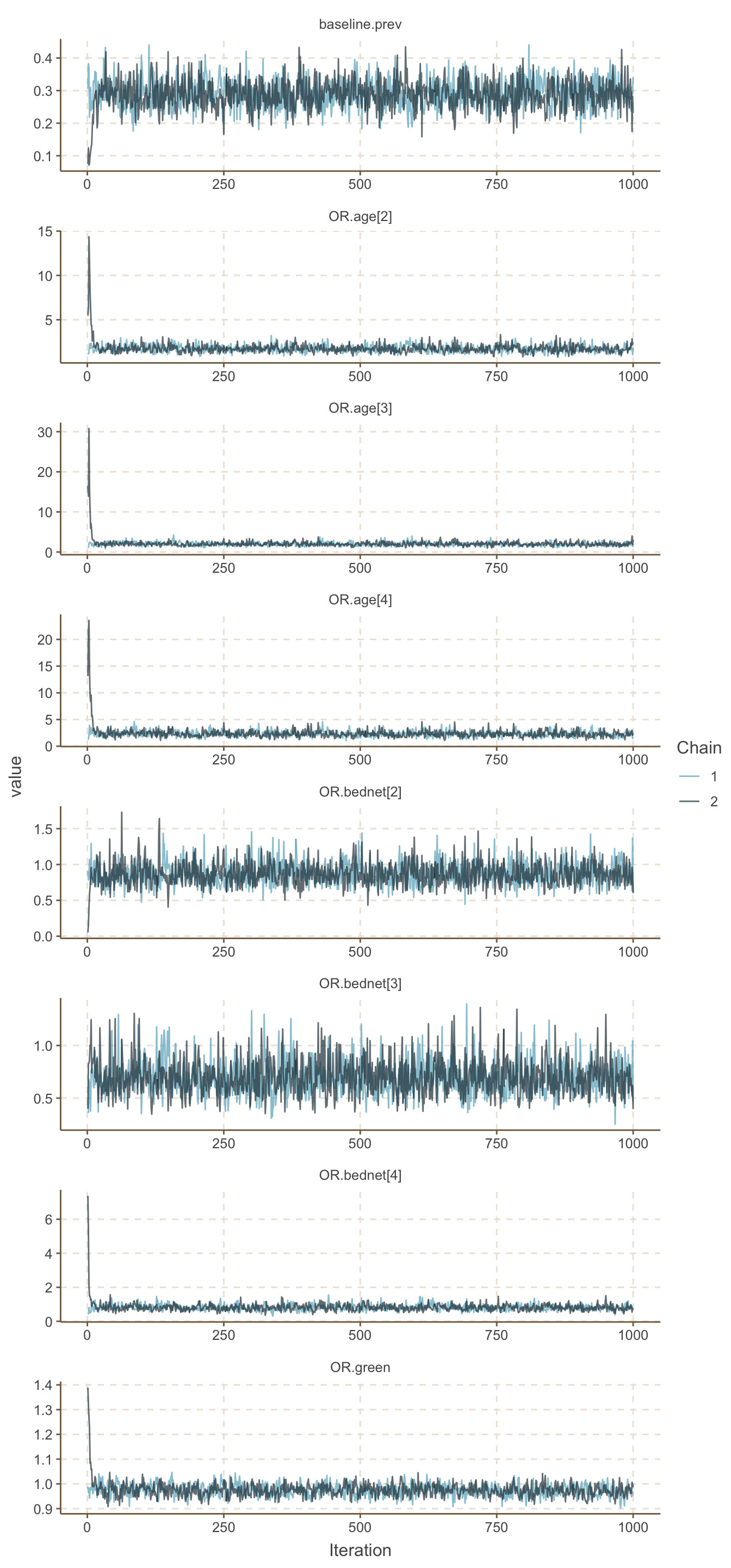

圖 101.1: Density plots for parameters for GLM about the odds of malaria regarding netbeds use in Gambia children.

## Potential scale reduction factors:
## 
##               Point est. Upper C.I.
## OR.age[2]          1.001       1.01
## OR.age[3]          1.009       1.03
## OR.age[4]          1.000       1.00
## OR.bednet[2]       1.000       1.01
## OR.bednet[3]       0.999       1.00
## OR.bednet[4]       1.001       1.01
## OR.green           1.003       1.01
## OR.phc             1.000       1.00
## PP.treated         1.003       1.01
## PP.untreated       1.002       1.01
## baseline.prev      1.000       1.00
## deviance           1.000       1.00
## 
## Multivariate psrf
## 
## 1.01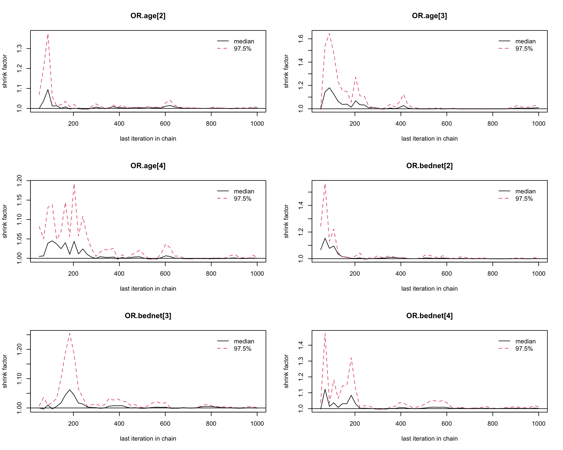

圖 101.2: Gelman-Rubin convergence statistic of parameters for GLM about the odds of malaria regarding netbeds use in Gambia children.

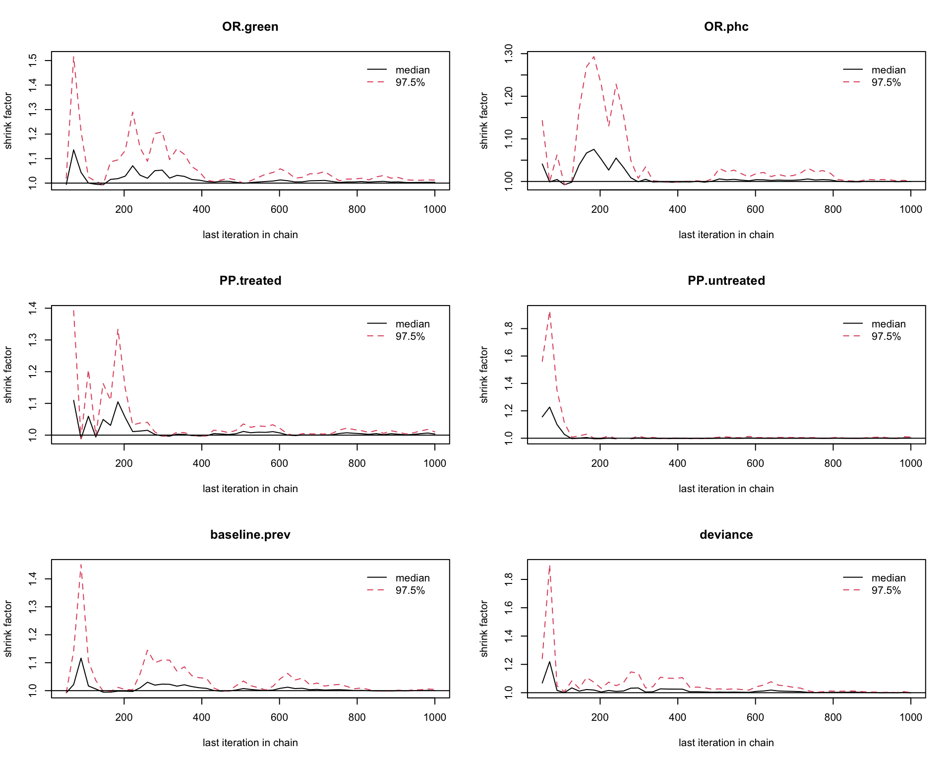
圖 101.3: Gelman-Rubin convergence statistic of parameters for GLM about the odds of malaria regarding netbeds use in Gambia children.

基本可以認爲刨除前1000次取樣 (burn-in) 可以達到收斂。

jagsModel <- jags(data = Dat,
                  model.file = paste(bugpath, 
                                  "/backupfiles/malaria-model-editted.txt",
                                  sep = ""),
                    parameters.to.save = parameters,
                     n.iter = 26000,
                     n.chains = 2, 
                     inits = inits,
                     n.burnin = 1000,
                     n.thin = 1,
                    progress.bar = "none")

## Compiling model graph
##    Resolving undeclared variables
##    Allocating nodes
## Graph information:
##    Observed stochastic nodes: 149
##    Unobserved stochastic nodes: 8
##    Total graph size: 1037
## 
## Initializing model

print(jagsModel)

## Inference for Bugs model at "/Users/chaoimacmini/Downloads/LSHTMlearningnote/backupfiles/malaria-model-editted.txt", fit using jags,
##  2 chains, each with 26000 iterations (first 1000 discarded)
##  n.sims = 50000 iterations saved
##               mu.vect sd.vect    2.5%     25%     50%     75%   97.5%  Rhat n.eff
## OR.age[2]       1.736   0.407   1.087   1.454   1.689   1.968   2.642 1.001 14000
## OR.age[3]       2.002   0.466   1.275   1.685   1.951   2.260   3.006 1.001 38000
## OR.age[4]       2.321   0.558   1.462   1.945   2.261   2.625   3.520 1.001 50000
## OR.bednet[2]    0.880   0.161   0.606   0.766   0.866   0.978   1.237 1.001 48000
## OR.bednet[3]    0.694   0.168   0.422   0.576   0.675   0.791   1.077 1.001  7300
## OR.bednet[4]    0.798   0.178   0.510   0.674   0.781   0.902   1.184 1.001 12000
## OR.green        0.975   0.024   0.930   0.959   0.975   0.991   1.022 1.001 50000
## OR.phc          0.712   0.130   0.491   0.621   0.701   0.792   0.999 1.001 17000
## PP.treated      0.877   0.328   0.000   1.000   1.000   1.000   1.000 1.001 50000
## PP.untreated    0.787   0.410   0.000   1.000   1.000   1.000   1.000 1.001 50000
## baseline.prev   0.288   0.043   0.208   0.258   0.286   0.316   0.377 1.001 49000
## deviance      461.068   5.795 455.179 458.084 460.358 463.242 470.614 1.049 50000
## 
## For each parameter, n.eff is a crude measure of effective sample size,
## and Rhat is the potential scale reduction factor (at convergence, Rhat=1).
## 
## DIC info (using the rule, pD = var(deviance)/2)
## pD = 16.8 and DIC = 477.9
## DIC is an estimate of expected predictive error (lower deviance is better).

參照組 (年齡小於2歲，不使用蚊帳，生活的村莊植被水平爲全部的平均值，且不在 PHC 管轄範圍內) 患瘧疾的百分比估計在 28.8% 左右 (baseline.prev)。極強的證據表明隨着年齡的增加，患瘧疾的危險度（比值）也升高。使用蚊帳可能可以降低一些些換瘧疾的危險度（比值），(OR.bednet[2] = 0.88) 但是其95%可信區間範圍是包括了1的 (0.605, 1.237)。使用未經殺蟲劑處理的蚊帳，也有79%的概率能夠降低兒童患瘧疾。和使用未經殺蟲劑處理的蚊帳相比，經過殺蟲劑處理的蚊帳也可能(有87.6%的概率)可以進一步降低兒童患瘧疾的危險 (OR.bednet[4] = 0.799, 95% 可信區間 0.51, 1.19)。和不在PHC管轄內的村莊相比，在PHC管轄的村莊可能可以降低兒童患瘧疾的危險 (OR.phc = 0.711，95% 可信區間 0.49, 0.99)。

把模型中發現和兒童發生瘧疾無太大關係的變量從貝葉斯邏輯迴歸模型中拿掉以後重新跑新的模型，和之前包含了全部變量的而模型相比較，你覺得哪個模型更合適？

由於植被指標變量和是否使用蚊帳的變量和是否發生瘧疾似乎關係不太大，我們把這兩個變量從模型中拿掉，再跑這個貝葉斯模型:

# Logistic regression model for malaria data
    
model {
   for(i in 1:149) {
      MALARIA[i] ~ dbin(p[i], POP[i])
      logit(p[i]) <- alpha + beta.age[AGE[i]] + beta.phc*PHC[i]  
   }
  
   # vague priors on regression coefficients
   alpha ~ dnorm(0, 0.00001)
   beta.age[1] <- 0          # set coefficient for baseline age group to zero (corner point constraint)
   beta.age[2] ~ dnorm(0, 0.00001)     
   beta.age[3] ~ dnorm(0, 0.00001)     
   beta.age[4] ~ dnorm(0, 0.00001)     
   beta.phc ~ dnorm(0, 0.00001)     
 
   # calculate odds ratios of interest
   OR.age[2] <- exp(beta.age[2]) # OR of malaria for age group 2 vs. age group 1
   OR.age[3] <- exp(beta.age[3]) # OR of malaria for age group 3 vs. age group 1
   OR.age[4] <- exp(beta.age[4]) # OR of malaria for age group 4 vs. age group 1
   
   OR.phc <- exp(beta.phc)      # OR of malaria sfor children living in villages belonging to the primary health care system versus children living in villages not in the health care system 
   logit(baseline.prev) <- alpha # baseline prevalence of malaria in baseline group (i.e. child in age group 1, sleeps without bednet, and lives in a village with average greenness index and not in the health care system) 
}

# Data file for the model
Dat <- list(
  POP = Data$POP, 
  MALARIA = Data$MALARIA, 
  AGE = Data$AGE, 
  PHC = Data$PHC
)


# initial values for the model
# the choice is arbitrary

inits <- list(
 list(alpha = -0.51, 
     beta.age = c(NA, 0.83,  0.28, -1.68), 
     beta.phc = 1.82),
 list(alpha = 1.29, 
      beta.age = c(NA, 0.49, -0.38, -0.04),  
      beta.phc = -0.31)
)



# Set monitors on nodes of interest
parameters <- c("OR.age", "OR.phc", "baseline.prev")

# fit the model in jags
jagsModel <- jags(data = Dat,
                  model.file = paste(bugpath, 
                                  "/backupfiles/malaria-model-dropped.txt",
                                  sep = ""),
                    parameters.to.save = parameters,
                     n.iter = 1000,
                     n.chains = 2, 
                     inits = inits,
                     n.burnin = 0,
                     n.thin = 1,
                    progress.bar = "none")

## Compiling model graph
##    Resolving undeclared variables
##    Allocating nodes
## Graph information:
##    Observed stochastic nodes: 149
##    Unobserved stochastic nodes: 5
##    Total graph size: 626
## 
## Initializing model

# Show the trace plot
Simulated <- coda::as.mcmc(jagsModel)
ggSample <- ggs(Simulated)
ggSample %>% 
  filter(Parameter %in% c("OR.age[2]", "OR.age[3]", "OR.age[4]", 
                          "baseline.prev")) %>% 
  ggs_traceplot()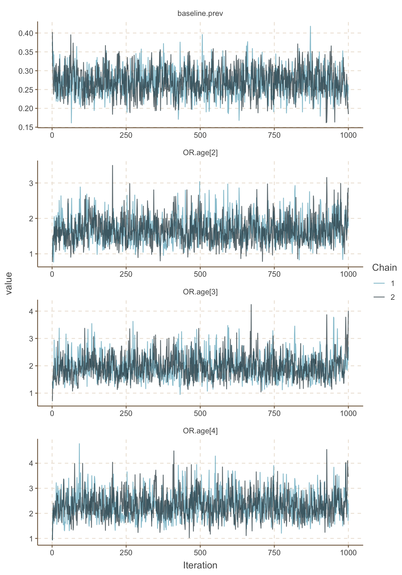

圖 101.4: Density plots for parameters for GLM about the odds of malaria regarding netbeds use in Gambia children.

## Potential scale reduction factors:
## 
##               Point est. Upper C.I.
## OR.age[2]           1.01       1.06
## OR.age[3]           1.00       1.01
## OR.age[4]           1.01       1.03
## OR.phc              1.00       1.00
## baseline.prev       1.01       1.04
## deviance            1.00       1.00
## 
## Multivariate psrf
## 
## 1.01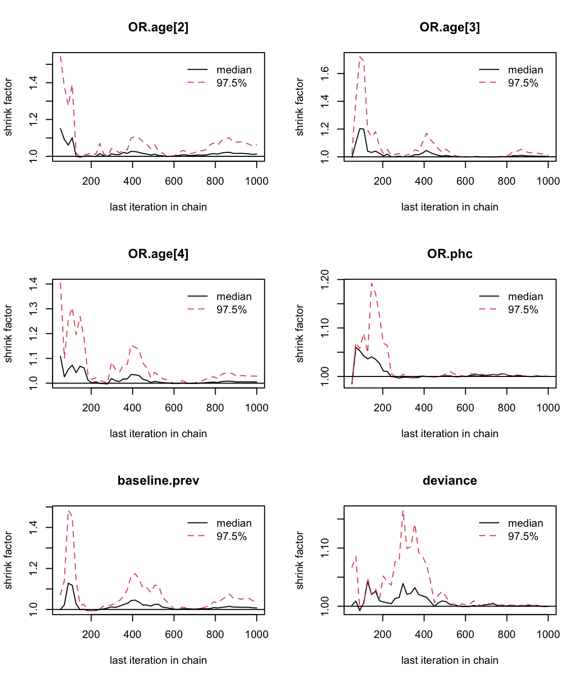

圖 101.5: Gelman-Rubin convergence statistic of parameters for GLM about the odds of malaria regarding netbeds use in Gambia children.

jagsModel <- jags(data = Dat,
                  model.file = paste(bugpath, 
                                  "/backupfiles/malaria-model-dropped.txt",
                                  sep = ""),
                    parameters.to.save = parameters,
                     n.iter = 26000,
                     n.chains = 2, 
                     inits = inits,
                     n.burnin = 1000,
                     n.thin = 1,
                    progress.bar = "none")

## Compiling model graph
##    Resolving undeclared variables
##    Allocating nodes
## Graph information:
##    Observed stochastic nodes: 149
##    Unobserved stochastic nodes: 5
##    Total graph size: 626
## 
## Initializing model

print(jagsModel)

## Inference for Bugs model at "/Users/chaoimacmini/Downloads/LSHTMlearningnote/backupfiles/malaria-model-dropped.txt", fit using jags,
##  2 chains, each with 26000 iterations (first 1000 discarded)
##  n.sims = 50000 iterations saved
##               mu.vect sd.vect    2.5%     25%     50%     75%   97.5%  Rhat n.eff
## OR.age[2]       1.680   0.382   1.058   1.408   1.638   1.905   2.554 1.001 50000
## OR.age[3]       1.964   0.435   1.261   1.652   1.916   2.221   2.946 1.001 50000
## OR.age[4]       2.316   0.524   1.466   1.944   2.255   2.625   3.505 1.001 40000
## OR.phc          0.651   0.106   0.469   0.577   0.643   0.717   0.881 1.001 15000
## baseline.prev   0.269   0.036   0.202   0.244   0.268   0.293   0.343 1.001 37000
## deviance      461.490   3.177 457.291 459.152 460.836 463.106 469.356 1.001 43000
## 
## For each parameter, n.eff is a crude measure of effective sample size,
## and Rhat is the potential scale reduction factor (at convergence, Rhat=1).
## 
## DIC info (using the rule, pD = var(deviance)/2)
## pD = 5.0 and DIC = 466.5
## DIC is an estimate of expected predictive error (lower deviance is better).

這個新模型的DIC和之間包含全部變量的模型相比降低了大概3左右，也就是去掉三個共變量對模型的影響。DIC的變化爲3時可認爲幾乎模型的擬合效果沒有太大的變化。出於簡約化模型的考慮，我們選擇這個新的變量較少的模型。

References

Diggle, Peter, Rana Moyeed, Barry Rowlingson, and Madeleine Thomson. 2002. “Childhood Malaria in the Gambia: A Case-Study in Model-Based Geostatistics.” Journal of the Royal Statistical Society: Series C (Applied Statistics) 51 (4): 493–506.