第 8 章 中心極限定理 the Central Limit Theorem
最近明顯可以感覺到課程的步驟開始加速。看我的課表:

手機畫面太小了。早上都是9點半開始,下午基本都是到5點。週一更慘,到7點。週二-週五中午都被統計中心的講座佔據。簡直是非人的生活。
這周概率論基礎結束。中心極限定理講完以後我們正式進入了 Inference 統計推斷的課程。我們花了一天時間講什麼是樣本估計 (Estimation),什麼是參數精確度 (Precision),什麼是自由度 (degree of freedom),怎樣進行不偏的估計 (unbiased inference)。然後還有似然方程 (likelihood function)。
今天的更新還是簡單的把概率論掃尾一下。感受一下中心極限定理的偉大。
8.1 協方差 Covariance
之前我們定義過,兩個獨立連續隨機變量 \(X,Y\) 之和的方差 Variance :
\[\text{Var}(X+Y)=\text{Var}(X)+\text{Var}(Y)\]
然而如果他們並不相互獨立的話:
\[ \begin{aligned} \text{Var}(X+Y) &= E[((X+Y)-E(X+Y))^2] \\ &= E[(X+Y)-(E(X)+E(Y))^2] \\ &= E[(X-E(X)) - (Y-E(Y))^2] \\ &= E[(X-E(X))^2+(Y-E(Y))^2 \\ & \;\;\; +2(X-E(X))(Y-E(Y))] \\ &= \text{Var}(X)+\text{Var}(Y)+2E[(X-E(X))(Y-E(Y))] \end{aligned} \]
可以發現在兩者和的方差公式展開之後多了一部分 \(E[(X-E(X))(Y-E(Y))]\)。 這個多出來的一部分就說明了二者 \((X, Y)\) 之間的關係。它被定義爲協方差 (Covariance): \[\text{Cov}(X,Y) = E[(X-E(X))(Y-E(Y))]\]
所以:
\[\text{Var}(X+Y)=\text{Var}(X)+\text{Var}(Y)+2Cov(X,Y)\]
要記住,協方差只能用於評價\(X,Y\)之間的線性關係 (Linear Association)。
以下是協方差 (Covariance) 的一些特殊性質:
- \(\text{Cov}(X,X)=\text{Var}(X)\)
- \(\text{Cov}(X,Y)=\text{Cov}(Y,X)\)
- \(\text{Cov}(aX,bY)=ab\:\text{Cov}(X,Y)\)
- \[\text{Cov}(aR+bS,cX+dY)=ac\:\text{Cov}(R,X)+ad\:\text{Cov}(R,Y)\\ \;\;\;\;\;\;\;\;\;\;\;\;\;\;\;\;\;\;\;\;\;\;\;\;\;\;\;\;\;\;\;\;\;\;\;\;\;+bc\:\text{Cov}(S,X)+bd\:\text{Cov}(S,Y)\]
- \[\text{Cov}(aX+bY,cX+dY)=ac\:\text{Var}(X)+ad\:\text{Var}(Y)\\ \;\;\;\;\;\;\;\;\;\;\;\;\;\;\;\;\;\;\;\;\;\;\;\;\;\;\;\;\;\;\;\;\;\;\;\;\;+(ad+bc)\text{Cov}(X,Y)\]
- \(\text{Cov}(X+Y,X-Y)=\text{Var}(X)-\text{Var}(Y)\)
- If \(X, Y\) are independent. \(\text{Cov}(X,Y)=0\) But not vise-versa !
8.2 相關 Correlation
- 協方差雖然\(\text{Cov}(X,Y)\) 的大小很大程度上會被他們各自的單位和波動大小左右。
- 我們將協方差標準化(除以各自的標準差 s.d.) (standardization) 之後,就可以得到相關係數 Corr (\(-1\sim1\)): \[\text{Corr}(X,Y)=\frac{\text{Cov}(X,Y)}{\text{SD}(X)\text{SD}(Y)}=\frac{\text{Cov}(X,Y)}{\sqrt{\text{Var}(X)\text{Var}(Y)}}\]
8.3 中心極限定理 the Central Limit Theorem
如果從人羣中多次選出樣本量爲 \(n\) 的樣本,並計算樣本均值, \(\bar{X}_n\)。那麼這個樣本均值 \(\bar{X}_n\) 的分佈,會隨着樣本量增加 \(n\rightarrow\infty\),而接近正(常)態分佈。
偉大的中心極限定理告訴我們:
當樣本量足夠大時,樣本均值 \(\bar{X}_n\) 的分佈爲正(常)態分佈,這個特性與樣本來自的人羣的分佈 \(X_i\) 無關。
再說一遍:
如果對象是獨立同分佈 i.i.d (identically and independently distributed)。那麼它的總體期望和方差分別是: \(E(X)=\mu;\;Var(X)=\sigma^2\)。 根據中心極限定理,可以得到:
- 當樣本量增加,樣本均值的分佈服從正(常)態分佈: \[\bar{X}_n\sim N(\mu, \frac{\sigma^2}{n})\]
- 也可以寫作,當樣本量增加: \[\sum_{i=1}^nX_i \sim N(n\mu,n\sigma^2)\]
- 有了這個定理,我們可以拋開樣本空間(\(X\))的分佈,也不用假定它服從正(常)態分佈。
- 但是樣本的均值,卻總是服從正(常)態分佈的。簡直是太完美了!!!!!!
8.5 泊松分佈的正(常)態分佈近似
假設時間 \(t\) 內某事件的發生次數服從泊松分佈 \(X\sim Po(\mu)\)。
考慮將這段時間 \(t\) 等分成 \(n\) 個時間段。那麼第 \(i\) 時間段內事件發生次數依舊服從泊松分佈 \(X_i\sim Po(\frac{\mu}{n})\)。且 \(E(X_i)=\mu/n, Var(X_i)=\mu/n\)。
那麼原先的 \(X\) 可以被視爲是將這無數的小時間段的 \(X_i\) 相加。應用中心極限定理: \[X=\sum_{i=1}^nX_i\sim N(\frac{n\mu}{n}, \frac{n\mu}{n})\]
需要注意的是,這段時間 (\(t\)) 內發生的事件次數 (\(\lambda\)) : \(\lambda t =\mu>10\) ,這樣的正(常)態分佈模擬才能成立。
8.6 正(常)態分佈模擬的校正:continuity corrections
- 如果我們使用正(常)態分佈來模擬離散變量的分佈,常常需要用到正(常)態分佈模擬的矯正。
- 例如:我們如果用正(常)態分佈模擬來計算 \(P(X=15)\),那麼實際上我們應該計算的是 \(P(14.5<X<15.5)\)。
8.6.1 例題
- 已知 \(X\sim Bin(100,0.5)\),求 \(P(X>60)\)
解
\[ \begin{aligned} \because X&\sim Bin(100, 0.5) \\ \therefore E(X) &=n\pi=50 \\ Var(X) &= n\pi(1-\pi) =25=5^2\\ P(X>60) &= 1-P(X\leqslant60) \\ &= 1-P(Z\leqslant\frac{60.5-50}{\sqrt{25}}) \\ &= 1-P(Z\leqslant2.1) \\ &= 1-\Phi(2.1) \\ &= 1-0.982 = 0.018 \end{aligned} \]
## [1] 0.0176## [1] 0.01786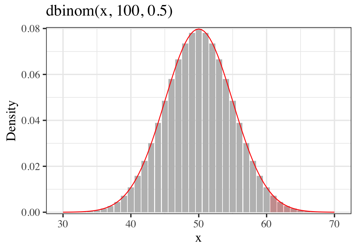
圖 8.1: Probability of 60 successes out of 100 Binomial trials, probability of success = 0.75
- 已知 \(X\sim Bin(48, 0.75)\), 求 \(P(30<X<39)\)
解
\[ \begin{aligned} \because B &\; \sim Bin(48, 0.75) \\ \therefore E(X) &\; =n\pi=36 \\ \text{Var}(X) &\; =n\pi(1-\pi)=9=3^2 \\ P(30<X<39) &\; = P(31\leqslant X\leqslant 38)\\ &\; = P(30.5\leqslant Y \leqslant 38.5) \\ Y\text{ is the }& \text{ normal approximation} \\ &\;= P(Y<38.5) - P(Y<30.5) \\ &\;= P(Z\leqslant\frac{38.5-36}{3})- P(Z\leqslant\frac{30.5-36}{3}) \\ &\;= P(Z\leqslant0.833) - P(Z\leqslant-1.833) \\ &\;= \Phi(0.833)-\Phi(-1.833) \\ &\;= 0.798-0.033 = 0.764 \end{aligned} \]
## [1] 0.7578## [1] 0.7643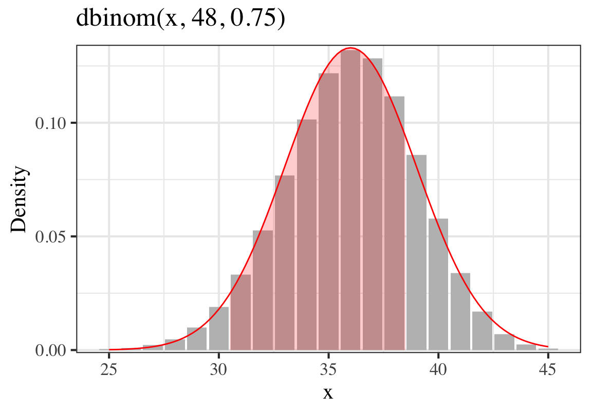
圖 8.2: Probability of 30-39 successes out of 48 Binomial trials, probability of success = 0.75
從上面兩個例題也能看出,\(n\) 越小,正(常)態分佈模擬的誤差就越大。
- 已知 \(X \sim Poisson(30)\) 求 \(P(X\leqslant20)\)。
解
\[ \because E(X)=\mu=30, \;Var(X)=\mu=30=(\sqrt{30})^2 \\ \begin{aligned} Pr(X\leqslant20) &= P(Z\leqslant\frac{20.5-30}{\sqrt{30}}) \\ &= P(Z\leqslant-1.734) \\ &= \Phi(-1.734) \\ &= 0.0414 \end{aligned} \]
## [1] 0.03528## [1] 0.04142這兩個其實有些小差距。不過看下圖,其模擬還是很到位的。只是正(常)態分佈的面積明顯確實比泊松分佈的小柱子面積要大一些。
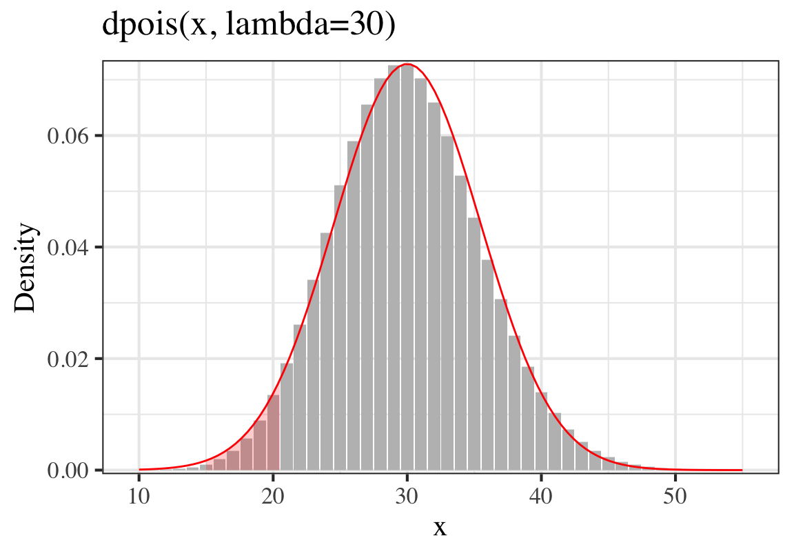
圖 8.3: Probability of less than 20 events happen when the expectation is 30
- 已知 \(X_1, X_2 \stackrel{i.i.d}{\sim} Poi(30)\) 求 \(P(X_1+X_2\leqslant40)\)。
解
\[ \begin{aligned} E(X_1+X_2) &\;= E(X_1)+E(X_2) = 30+30 = 60\\ Var(X_1+X_2) &\;= Var(X_1)+Var(X_2) = 30+30 \\ &\;= (\sqrt{60})^2 \\ P(X_1+X_2\leqslant 40) &\;= P(Z \leqslant \frac{40.5-60}{\sqrt{60}}) \\ &\;= P(Z\leqslant-2.517) \\ &\;= \Phi(-2.517) \\ &\;= 0.006 \end{aligned} \]
## [1] 0.003983## [1] 0.005911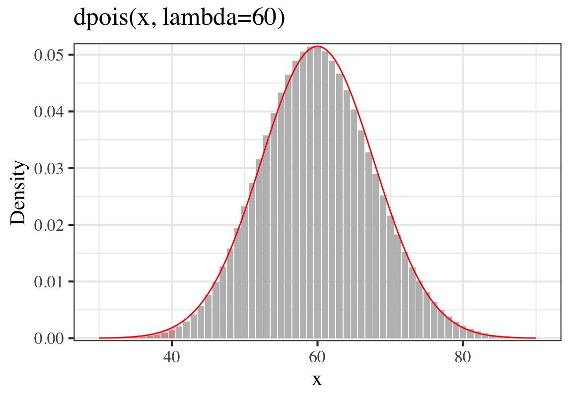
圖 8.4: Probability of 2 identically and independently observed results of less or equal to 40 events happen in total when the expectation of each observation is 30
又一次,正(常)態分佈的面積比泊松分佈的小柱子面積要大一些。
8.7 兩個連續隨機變量
假定 \(X_1, X_2\) 是兩個連續隨機變量: \[ E(X_1)=\mu_1, \text{Var}(X_1)=\sigma_1^2 \\ E(X_2)=\mu_2, Var(X_2)=\sigma_2^2 \\ Corr(X_1, X_2)=\rho \Rightarrow \text{Cov}(X_1, X_2)=\rho\sigma_1\sigma_2=\sigma_{12} \]
利用矩陣的標記法,可以將 \(X_1, X_2\) 標記爲 \(\textbf{X}=(X_1, X_2)^T\), 即:
\[ \textbf{X}=\left( \begin{array}{c} X_1\\ X_2\\ \end{array} \right) \]
- 上面的所有內容都可以標記爲: \[ E(\textbf{X})=\mathbf{\mu}=\left( \begin{array}{c} \mu_1\\ \mu_2\\ \end{array} \right)\\ Covariance \;matrix: \\ Var(\textbf{X})=\mathbf{\Sigma}=\left( \begin{array}{c} \sigma_1^2 & \sigma_{12}\\ \sigma_{12} & \sigma_2^2\\ \end{array} \right) \]
8.8 兩個連續隨機變量 例子:
假如要看收縮期血壓 (\(SBP\)) 和舒張期血壓 (\(DBP\)) 之間的關係:
下列爲已知條件:
- \(SBP\) 的均值爲 \(130\), 標準差爲 \(15\);
- \(DBP\) 的均值爲 \(90\), 標準差爲 \(10\);
- \(SBP\) 和 \(DBP\) 之間的相關係數爲 \(0.75\)。
那麼, 我們可以把這些信息用下面的方法來標記:
\[ E(\textbf{X})=\mathbf{\mu}=\left( \begin{array}{c} 130\\ 90\\ \end{array} \right)\\ Var(\textbf{X})=\mathbf{\Sigma}=\left( \begin{array}{c} 15^2 = 225 & 0.75 \times 15 \times 10 = 112.5\\ 0.75 \times 15 \times 10 = 112.5 & 10^2 = 100\\ \end{array} \right) \]
8.9 條件分佈和邊緣分佈的概念
如果 \(\textbf{X}=(X_1, X_2)^T\) 的兩個變量都服從正(常)態分佈;
那麼這兩個變量的邊緣分佈 (marginal distribution) 也服從正(常)態分佈: \[X_1\sim N(\mu_1,\sigma_1^2), X_2\sim N(\mu, \sigma_2^2)\]
同樣的,\(X_1\) 的給出 \(X_2\) 的條件分佈 (condition distribution) 也服從正(常)態分佈: \[E(X_1|X_2)=\mu_1+\frac{\rho\sigma_1}{\sigma_2}(X_2-\mu_2) \\ \text{Var}(X_1|X_2)=\sigma_1^2(1-\rho^2)\]
反之亦然。
8.10 條件分佈和邊緣分佈的例子
上面的概念過於抽象,用血壓的例子:
收縮期血壓和舒張期血壓各自服從正(常)態分佈。那麼可以用上面的概念來寫出已知舒張期血壓時,收縮期血壓的分佈。
條件期望: \[E(\text{SBP|DBP})=130+\frac{0.75\times15}{10}(\text{DBP}-90)\]
實際如果來了一個病人,他說他只記得自己測的舒張期血壓是95:
他的收縮期血壓的期望值就可以用上面的式子計算: \[E(\text{SBP|DBP}=95)=136\]條件方差爲: \[\text{Var}(\text{SBP|DBP})=15^2(1-0.75^2)=98.4\approx9.92^2<15^2\]
所以當我們知道了這個人的一部分信息以後,推測他的另一個相關連的變量變得更加準確(方差變小)了。
8.10.1 例題
有 (閒) 人記錄了 \(1494\) 名兒童在 \(2, 4, 6\) 歲時的腿長度。已知在記錄的這三個年齡時的平均腿長度分別爲 \(85 \text{ cm}, 103 { cm}, 114 { cm}\)。協方差矩陣如下:
\[ \left( \begin{array}{c} 22.2 & 11.8 & 13.7\\ 11.8 & 26.3 & 21.5\\ 13.7 & 21.5 & 29.0 \end{array} \right) \]
假定,這三個年齡記錄的這些兒童的腿長度數據(聯合分佈, joint distribution)服從三個變量正(常)態分佈。
- 求 \(2\) 歲時這些兒童的腿長度的邊緣分佈 (marginal distribution)
解
\[X_{\text{age}=2} \sim N(85, \sigma_{\text{age}=2}^2=22.2)\]
- 求他們 \(6\) 歲時腿長度的 \(2\) 歲時的條件分佈。(Find the distribution of leg length age 6 conditional on leg length at age 2.)
解
\(6\) 歲時和 \(2\) 歲時腿長的相關係數 (correlation, \(\rho_{6,2}\)) 爲:
\[ \begin{aligned} \rho_{6,2} &= \frac{Cov_{6,2}}{\sqrt{\text{Var}(\text{length}_6)}\sqrt{\text{Var}(\text{length}_2)}}\\ &= \frac{13.7}{\sqrt{22.2}\sqrt{29}}=0.54 \end{aligned} \]
條件分佈套用上面提到的公式:
\[ \begin{aligned} E({\text{length}_6 | \text{length}_2}) &= \mu_6+\frac{\rho_{6,2}\sigma_6}{\sigma_2}(\text{length}_2-\mu_2) \\ &= 114+\frac{0.54\times\sqrt{29.0}}{\sqrt{22.2}}(\text{length}_2-85)\\ \text{Var}(\text{length}_6 | \text{length}_2) &= \sigma_6^2(1-\rho_{6,2}^2) \\ &= 29.0\times(1-0.54^2) =20.5 \end{aligned} \]