第 96 章 蒙特卡羅估計和預測 Mente Carlo estimation and prediction
96.1 起源
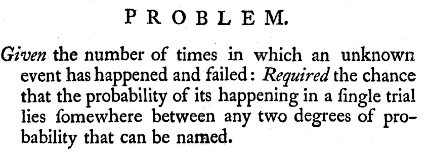
圖 96.1: Reproduction of part of the original printed Bayes paper.
一切都開始於1763年,英國東南地區叫做唐橋井 (Tunbridge Wells) 的地方有個叫做託馬斯貝葉斯的牧師死後,他的朋友將他遺留下的手稿發表於世。圖 96.1 是他遺作論文的節選。這段話使用的當時的英文有點令人摸不着頭腦,但其實翻譯成現代文的意思是(這裏請在大腦中想象我們最長使用的投擲一枚可能有偏的硬幣的場景):我們一共投擲硬幣 \(n\) 次,這其中有 \(y\) 次硬幣是正面朝上的(事件發生)。假定 \(y\) 服從參數爲 \(\theta\) 的二項分布:\(y \sim \text{Binomial}(\theta, n)\),那麼\(\theta\)就是硬幣正面朝上的概率。
貝葉斯牧師感興趣的是,參數\(\theta\),落在某個範圍內 \(\text{Pr}(\theta_1 < \theta < \theta_2 | y, n)\)的可能性(chance)。這句話,在當年那個概率論持有者爲主流的社會中是極爲危險而且激進的 (radical) ,因爲貝葉斯牧師使用可能性 (chance)來描述一個參數的不確定性(uncertainty)。本質上說,貝葉斯牧師打算對一個無法直接觀測的參數用一個簡單直接的數學表達式來描述它的不確定性。這句話對於概率論觀點持有者佔主流的統計學領域來說,是一種明顯的異端邪說。因爲在概率論觀點持有者的語境下,概率是在無數次可重復實驗中事件發生的平均次數 (probability is interpreted in terms of a long run sequence of events),這個無法觀測到的參數,是不會改變的 (the key idea is that the unknown parameter is considered to be a random variable under Bayesian theory, rather than fixed but unknown)。
我們在第一章也看到了,貝葉斯牧師提出的理論有助於我們直接,正面地回答研究中我們想知道的問題。圖 96.2 提供了一個很好的例子,它節選自論文(Tinmouth et al. 2004)中,該文的作者是這樣描述的:“There is an 89% probability that the absolute increase in major bleeds is less than 10 percent with low-dose PLT transfusions. (使用低劑量PLT輸血時,患者大出血的出血量增加的絕對值小於10%的可能性是89%。)”
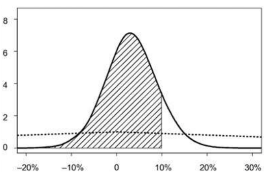
圖 96.2: Example of a direct expression about an unknown parameter.
像圖 96.2 這樣使用一個概率分布來描述我們想知道的參數有什麼好處呢?
- 最重要的好處是,用概率分布描述這個未知參數可以直觀地告訴我們這個參數它本身可能分布的範圍,和在各自分布點時的可能性。
- 沒有 p 值,因爲我們要計算整個參數可能分布的範圍,這是概率密度分布的面積。
- 沒有(難以令人理解的)信賴區間的概念(confidence interval),相反地,我們需要盡可能詳細地描述參數可能的分布,它的中位數,它的均值,它可能取值的範圍,它中間包含了95%可信範圍的參數(credible interval)
- 方便地直接應用於預測。
- 自然地適用於決策分析 (decision analysis),經濟學的成本效益分析 (cost-effective analysis)等。
- 貝葉斯理論讓我們從數學上把經驗(已經發表的實驗結果,以及已有的專家意見)納入到參數的估計上來,這是一個自我學習進化的過程。
96.2 百分比的統計學推斷 inference on proportions
我們先用一個新藥的臨牀試驗來作爲例子。
96.2.1 Example: New Drug
有一種新研發的被用於治療慢性疼痛的藥物。爲了對其有效性進行科學客觀的評價,研究者需要組織一項評價其效用的小規模臨牀試驗。在實施這項臨牀試驗之前,我們自己心裏就會提出一個問題,這個新藥物用於治療慢性疼痛時有療效的百分比有可能會是多少(期望值,expectation)?
假如經驗告訴我們,相似成分的藥物可能達到的有療效百分比是在0.2-0.6之間。那麼我們可以把這個經驗翻譯成爲,有效率的期望可能服從某個分布,其均值是0.4,標準差是 0.1,下一步就是用一個能夠具有這樣的均值和標準差特徵的分布來表達這個經驗。我們在數學的寶庫中發現了 Beta 分布這個可以用於描述百分比的分布。
96.2.2 Beta 分布
Beta 分布的特徵是取值範圍嚴格限定在0, 1之間,這就滿足了百分比數值的取值範圍條件。它由兩個參數來決定分布的特徵。
我們用 \(\theta \sim \text{Beta}(a, b)\) 標記 Beta 分布。它的特徵值有:
\[ \begin{aligned} p(\theta|a, b) & = \frac{\Gamma(a + b)}{\Gamma(a)\Gamma(b)}\theta^{a-1}(1-\theta)^{b-1}; \theta \in (0,1) \\ \text{E}(\theta|a, b) & = \frac{a}{a+b} \\ \text{V}(\theta|a, b) & = \frac{ab}{(a+b)^2(a + b + 1)} \end{aligned} \]
其中 \(\Gamma(a) = (a-1)!\) 是一個伽瑪方程。
正如我們在貝葉斯入門的章節42.3.1也介紹過的那樣,Beta分布的一些形狀特徵總結如下:
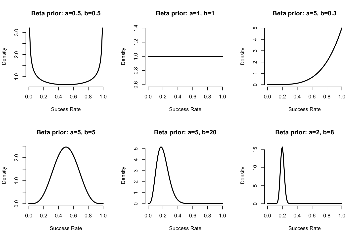
圖 96.3: Shape of some Beta distribution functions for various values of a, b
回到新藥試驗的話題上來看,我們的經驗被翻譯成了均值爲0.4, 標準差0.1,那麼把它們帶入Beta分布的均值方差的特徵值公式中去,就可以求得相對應的Beta分布:\(\text{Beta}(9.2, 13.8)\)
\[ \begin{aligned} \theta & \sim \text{Beta}(9.2, 13.8) \\ \text{E}(\theta) & = \frac{9.2}{9.2 + 13.8} = 0.4 \\ \text{V}(\theta) & = \frac{9.2\times13.8}{(9.2 + 13.8)^2(9.2+13.8+1)} = 0.01 = 0.1^2 \end{aligned} \]
這個本來只是一句話的經驗,就被我們成功用Beta分布翻譯成了數學模型可以使用的分布方程,它的概率密度曲線如下,使用這個Beta分布的含義就是,經驗告訴我們相似成分的藥物可能達到的有療效百分比是在0.2-0.6之間:
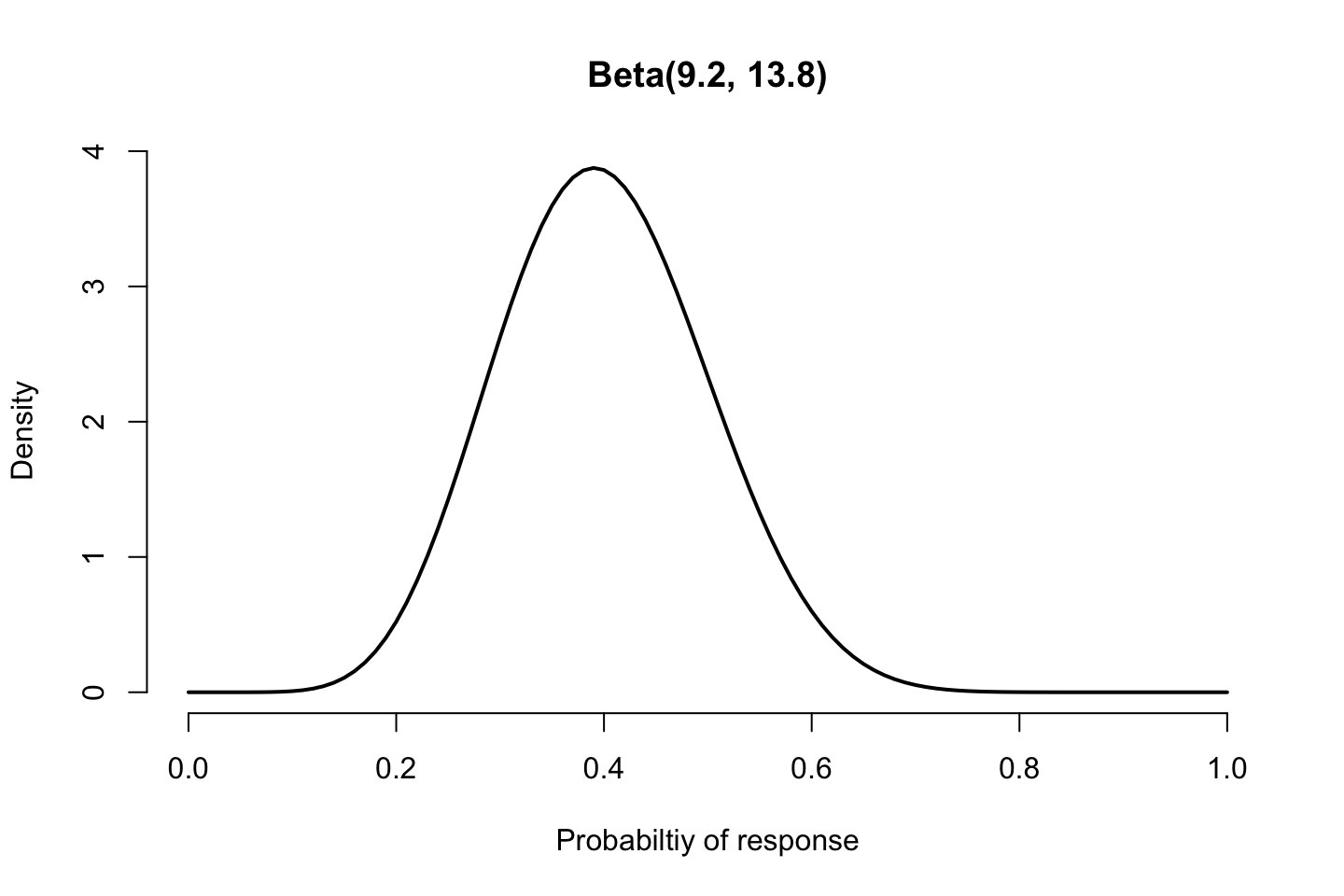
圖 96.4: Prior distribution for Drug Example
96.2.3 作出預測
在臨牀試驗觀測到有療效人數 \(y\) 之前,我們可以通過把未知參數積分消除(intergrate out)的方法給出預測分布:
\[ p(y) = \int p(y|\theta)p(\theta)d\theta \]
預測在很多領域都可以得到廣泛的應用,比如做天氣預報,經濟學上的成本效益分析,進行實驗設計,以及用於檢驗觀測數據是否和期望值相匹配,等等。
96.2.4 Example: 新藥表現預測
我們再回到新藥治療慢性疼痛的臨牀試驗上來,假設我們設計接納20名患者進入這個臨牀試驗。那麼我們可能想根據已有的經驗,來預測一下這進來的20名患者中藥物有效的人數。
我們已經知道用 Beta 分布來描述經驗(也就是先驗概率 prior distribution),此時,我們再加入用 \(y\) 標記20名患者中有效人數的隨機變量。那麼很自然地,我們會使用二項分布作爲 \(y\) 的理想模型:
\[ \begin{aligned} \theta & \sim \text{Beta} (a,b) \\ y & \sim \text{Binomial}(\theta, n) \end{aligned} \]
這個模型的預測模型能夠被計算得到(甚至不需要用到計算機),且它有個自己的專有名字 Beta-Binomial,它的概率方程是:
\[ \begin{aligned} p(y) & = \frac{\Gamma(a+b)}{\Gamma(a)\Gamma(b)}\binom{n}{y}\frac{\Gamma(a + y)\Gamma(b + n - y)}{\Gamma(a + b + n)} \\ & = \binom{n}{y}\frac{B(a + y, b + n -y)}{B(a,b)} \end{aligned} \] 其中,\(B(a,b) = \frac{\Gamma(a)\Gamma(b)}{\Gamma(a+b)}\);
均值是:
\[ \text{E}(Y) = n\frac{a}{a + b} \]
那麼我們在進行這項試驗時我們可以預測,20名患者中有療效人數出現的概率,我們將它的預測概率分布圖和先驗概率分布放在一起:
# # Beta Binomial Predictive distribution function
# BetaBinom <- Vectorize(function(rp){
# log.val <- lchoose(np, rp) + lbeta(rp+a+r,b+n-r+np-rp) - lbeta(a+r,b+n-r)
# return(exp(log.val))
# })
par(mfrow=c(1,2))

pi <- Vectorize(function(theta) dbeta(theta, 9.2,13.8))
curve(pi, xlab="Probabiltiy of response", ylab="Density", main="(a) Prior distribution Beta(9.2, 13.8)", frame=FALSE, lwd=2)

# or we can use the built-in function for beta-binomial distribution in package TailRank:
library(TailRank)
N <- 20; a <- 9.2; b <- 13.8; y <- 0:N
yy <- dbb(y, N, a, b)
barplot(yy, xlab = "Number of successes", names.arg = 0:20, axes = F,
        ylim = c(0, 0.16), main = "(b) predictive distribution")
axis(2,at=seq(0,0.16,0.02))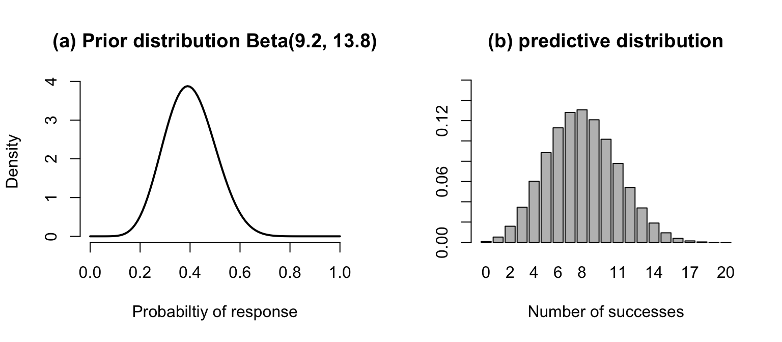
圖 96.5: Prior and predictive distribution for the drug example.
我們根據這個預測概率分布,或者預測概率方程,可以計算”20名患者中有15名或者更多的患者的症狀得到改善”這一事件出現的概率會是:
\[ P(y \geqslant 15) = \sum_{15}^{20}p(y) = 0.015 \]
96.3 蒙特卡羅估計
但是在一般的情況下,像這個新藥臨牀試驗這樣能夠獲得一個閉環式 (closed-form) 概率預測概率方程的情況少之又少,有時候幾乎是不太可能完成的任務。假設我們本來也無法順利計算出上面的 Beta-Binomial概率公式,我們是否有其他的手段來獲得我們想要的預測概率結果呢?答案是,有的。人類發明的計算機,可以通過模擬試驗的方式(computer simulation)幫我們計算這個結果,它有個很酷的名字,叫做蒙特卡羅積分 (Monte Carlo integration)。
96.3.1 用蒙特卡羅法估計概率分佈尾側累積概率(面積)
假設要求一個很簡單的問題,一枚完美的硬幣,投擲10次中8次甚至更多次正面朝上的概率是多少?
在概率數學上,我們會用正式的方法來求:
\[ \begin{aligned} y & \sim \text{Binomial}(0.5, 10), \text{Pr}(y \geqslant 8)? \\ \text{Pr}(y\geqslant 8 \text{ heads}) & = \sum_{y = 8}^{10}p(y | \theta = 0.5, n = 10) \\ & = \binom{10}{8}(0.5)^8(0.5)^2 + \binom{10}{9}(0.5)^9(0.5)^1 + \binom{10}{10}(0.5)^{10}(0.5^0) \\ & = 0.0547 \end{aligned} \]
但是,如果有人很懶,他可以不這樣計算,而是真的拿那個硬幣過來不停的進行很多很多次投擲試驗,然後計算其中8次正面朝上出現的試驗的比例,那麼從長遠來說,就能夠無線接近理論計算的概率數值。
那麼,計算機進行模擬試驗的過程 (simulation),其實就是讓計算機代替我們進行投擲硬幣試驗的過程。圖 96.6 展示的是計算機模擬投擲硬幣(a) 100次 (b) 10,000 次時正面朝上次數的概率分佈,以及 (c) 真實的概率分佈。
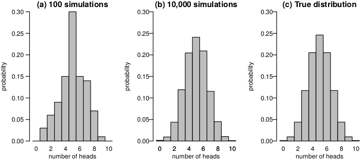
圖 96.6: Proportion of simulations with 8 or more “heads” in 10 tosses.
從中可以計算每種情況下硬幣正面朝上10次中出現8次或者更多的事件出現的概率分別是:
- 100次模擬試驗: 0.08
- 10000次模擬試驗: 0.0562
- 真實的二項分佈累積概率: 0.0547
可見,當模擬試驗的次數增加,計算想要的事件出現的比例,就越來越接近理論計算的真實值。蒙特卡羅積分法,用的也是類似計算機模擬試驗的方法來計算預測概率分佈的。
96.3.2 用蒙特卡羅法計算預測概率分佈
如果用蒙特卡羅法,也就是計算機模擬試驗的方法來計算預測概率分佈的話,那麼我們就不需要再通過 Beta-binomial 概率分佈的公式來進行計算了。取而代之的就是,蒙特卡羅積分法:
- 從先驗概率分佈中隨機選取一個值 \(\theta = \theta_1\)
- 把從先驗概率分佈中隨機選取的 \(\theta_1\) 作爲已知量放到二項分佈中再隨機選取一個服從 \(n = 20, \theta = \theta_1\) 二項分佈數據中的 \(y\)。
重複上面步驟1,2成千上萬次之後,獲得的新的概率分佈,就是 \(y\) 的預測分佈的一個樣本。這樣獲得的樣本,我們就可以想進各種方法來描述它,可以是取均值,取方差,取四分位,等任何你可以用來描述的特徵值來作爲對預測概率分佈的描述。
96.4 蒙特卡羅法分析軟件 OpenBUGS / JAGS
本書中我們主要用 JAGS 軟件進行貝葉斯統計分析。
96.4.1 用 JAGS/BUGS 分析投擲硬幣數據
回到投擲硬幣的簡單模型上來,我們的隨機變量 \(y\) 服從的是二項分佈,\(y \sim \text{Binomial}(0.5, 10)\),我們想要計算的是”8次或者更多次正面朝上”事件出現的概率: \(P(y\geqslant 8)\)。這一模型在 BUGS 語言下被描述爲:
model{
    y ~ dbin(0.5, 10)
    P8 <- step(y - 7.5)
}其中step是一個能夠產生邏輯結果(True or False)的指示方程(indicator function)。P8 <- step(y - 7.5)這段BUGS語句的含義是,當y - 7.5的結果\(\geqslant0\),P8將會取 1 (True),反之將返回結果 0 (False)。意思就是使得當隨機選取的二項分布樣本 \(y\geqslant8\) 時,P8會取值1,否則取0。
將這一段計算機模擬拋擲硬幣的語句重復一萬次以上(iterations),然後對獲得的所有10000個P8取均值,獲得的就會是 \(y\geqslant8\) 這一事件將會出現的概率。
96.4.2 用 JAGS 對藥物臨牀試驗的結果做預測
還記得我們在藥物對慢性疼痛治療療效評價的這一臨牀試驗中使用的先驗概率是 \(\theta \sim \text{Beta}(9.2, 13.8)\)。我們再來思考一次,我們收集到20位志願者參加這個臨牀試驗,那麼”這20位患者中,有15名或者更多的患者症狀得到改善(治療有效)“這件事發生的概率是多少?
這時候,模型的先驗概率和似然,以及我們想要知道的問題,被數學語言寫成了下面的三句話:
\[ \begin{split} \theta & \sim \text{Beta}(9.2, 13.8) & \text{ Prior distribution} \\ y & \sim \text{Binomial}(\theta, 20) & \text{ Sampling distribution} \\ P_{crit} & = P(y \geqslant 15) & \text{ Probability of exceeding critical threshold} \end{split} \]
如果要把這三句話翻譯成爲JAGS的BUGS語言,可以這樣表達:
model{
  theta ~ dbeta(9.2, 13.8) # Prior distribution
  y ~ dbin(theta, 20)      # Sampling distribution
  P.crit <- step(y - 14.5) # = 1 if y >= 15, 0 otherwise
}
計算機模擬試驗10000次以後獲得的結果可能是下面這樣子的
Node statistics
          mean      sd       MC_error    val2.5pc    median  val97.5pc  start   sample
P.crit  0.015      0.1216      0.00121   0.0         0.0       0.0        1       10000
theta   0.4008   0.09903     9.683E-4    0.2159    0.3982    0.5993     1       10000
y 8.034 2.919 0.02578 3.0 8.0 14.0 1 10000第一行我們可以看見顯示的是列的名稱,接下來每一行都是JAGS/OpenBUGS的軟件在進行計算機模擬試驗過程中監測的(monitor)變量的結果,以及它們的數據描述。值得注意的是其中P.crit這一行,除了第一列的均值mean = 0.015有實際意義意外,其餘的數值是沒有什麼含義的,可以忽略。這個P.crit均值的含義即是我們關心的問題【“這20位患者中,有15名或者更多的患者症狀得到改善(治療有效)”這件事發生的概率】的答案,是0.015。
我們可以把蒙特卡羅算法給出的計算機模擬試驗的結果,和精確統計學計算法獲得的結果相比較:
- \(\theta:\) 均值0.4,標準差0.1;
- \(y:\) 均值8, 標準差2.93。
- 20人中15人及以上治療有效的概率是0.015。
由於這些樣本是互相獨立的,輸出結果中的 MC_error \(=\frac{\text{SD}}{\sqrt{\text{n of iterations}}}\)。如果你願意,完全可以爲了提高精確度再增加計算機模擬試驗的次數。
OpenBUGS 同時可以輸出計算機模擬計算過後的圖片:
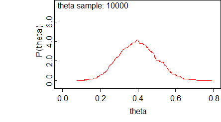
圖 96.7: Example OpenBUGS plots from the drug example
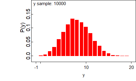
圖 96.8: Example OpenBUGS plots from the drug example
96.4.3 用蒙特卡羅法計算一個臨牀試驗的統計效能 allow uncertainty in power calculation
假設有一個臨牀試驗是這樣設計的,計劃在治療組和對照組各徵集 \(n\) 名患者,治療陽性反應率的標準差爲\(\sigma = 1\)。設計上希望達到一類錯誤 5%,和80%的效能。治療組和對照組的療效差異希望能達到 \(\theta = 0.5\)。計算樣本量爲\(n\),療效差爲\(\theta\)的試驗的統計效能的數學公式已知爲:
\[ \text{Power} = \Phi(\sqrt{\frac{n\theta^2}{2\sigma^2}} - 1.96) \]
再假設我們希望對\(\theta,\sigma\)同時描述其不確定性:
\[ \begin{aligned} \theta & \sim \text{Uniform}(0.3, 0.7) \\ \sigma & \sim \text{Uniform}(0.5, 1.5) \\ \end{aligned} \]
接下來,我們可以利用這個公式和給出的先驗概率對統計效能的不確定性進行估計。
- 模擬從\(\theta, \sigma\)的先驗概率中各自選取相應的值;
- 把每次模擬試驗獲得的 \(\theta, \sigma\) 代入上面計算效能的公式中計算每次可以獲得的統計效能;
- 重復步驟1,2許多次,獲取這個過程中計算得到的統計效能的預測分布(predictive distribution)。
如果說每組患者人數是63人,那麼這個模型寫成BUGS語言就是:
model{
  sigma ~ dunif(0.5, 1.5)
  theta ~ dunif(0.3, 0.7)
  power <- phi(sqrt(63/2)*theta/sigma - 1.96)
  prob70 <- step(power - 0.7) # is power >= 0.7
}該模型的輸出結果如下,預測的效能分布圖爲圖96.9:
Node statistics
         mean     sd       MC_error   val2.5pc   median   val97.5pc   start   sample
power    0.7508   0.2249   0.00216    0.2846     0.8031   1.0         1       10000
prob70   0.6265   0.4837   0.004626   0.0        1.0      1.0         1       10000
當治療組對照組每組各只有63人時,你會發現統計效能在電腦模擬10000次試驗過後的中位數才勉強達到了80%,而且這麼寬的效能預測分布也提示我們63人實在太少了,效能遠遠不能達到設計的要求。
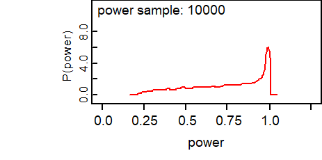
圖 96.9: Predictive Distribution of Power
96.5 Practical Bayesian Statistics 02
- 拋擲硬幣試驗
用BUGS語言描述拋擲硬幣的模型,把寫有下列模型代碼的文件保存爲coinmodel.txt:
model{
  y ~ dbin(0.5, 10)
  P8 <- step(y - 7.5) # = 1 if Y is 8 or more
}
下面的代碼展示了如何在 R 裏連接OpenBUGS進行蒙特卡羅運算和調出其結果的過程:
library(BRugs)

# Step 1 check model
modelCheck(paste(bugpath, "/backupfiles/coinmodel.txt", sep = ""))
# there is no data so just compile the model
modelCompile(numChains = 1)
# There is no need to provide initial values as this is
# a Monte Carlo forward sampling from a known distribution
# but the program still requires initial values to begin
# generate a random value.
modelGenInits() #
# Set monitors on nodes of interest
samplesSet(c("P8", "y"))
# Generate 1000 iterations
modelUpdate(1000)

#### SHOW POSTERIOR STATISTICS
sample.statistics <- samplesStats("*")
print(sample.statistics)

#### PUT THE SAMPLED VALUES IN ONE R DATA FRAME:
chain <- data.frame(P8 = samplesSample("P8"),
                    y = samplesSample("y"))
samplesHistory("*", mfrow = c(2,1), ask=FALSE)
下面的代碼展示了如何在R裏連接JAGS進行蒙特卡羅運算和調出其結果的過程:
library(runjags)
library(rjags)
library(R2jags)

# Step 1 check model
jagsModel <- jags.model(file = paste(bugpath, "/backupfiles/coinmodel.txt", sep = ""), n.chains = 1)
## Compiling model graph
## Resolving undeclared variables
## Allocating nodes
## Graph information:
## Observed stochastic nodes: 0
## Unobserved stochastic nodes: 1
## Total graph size: 6
##
## Initializing model# Step 2 update 1000 iterations
update(jagsModel, n.iter = 1000, progress.bar="none")
# Step 3 set monitor variables
codaSamples <- coda.samples(
jagsModel,
variable.names = c("P8", "y"),
n.iter = 1000, progress.bar="none")
summary(codaSamples)##
## Iterations = 1001:2000
## Thinning interval = 1
## Number of chains = 1
## Sample size per chain = 1000
##
## 1. Empirical mean and standard deviation for each variable,
## plus standard error of the mean:
##
## Mean SD Naive SE Time-series SE
## P8 0.058 0.23386 0.0073953 0.0073953
## y 4.941 1.57226 0.0497191 0.0497191
##
## 2. Quantiles for each variable:
##
## 2.5% 25% 50% 75% 97.5%
## P8 0 0 0 0 1
## y 2 4 5 6 8# Show the trace plot
# library(mcmcplots)
# ggSample <- ggs(codaSamples)
# ggs_traceplot(ggSample)
mcmcplots::traplot(codaSamples)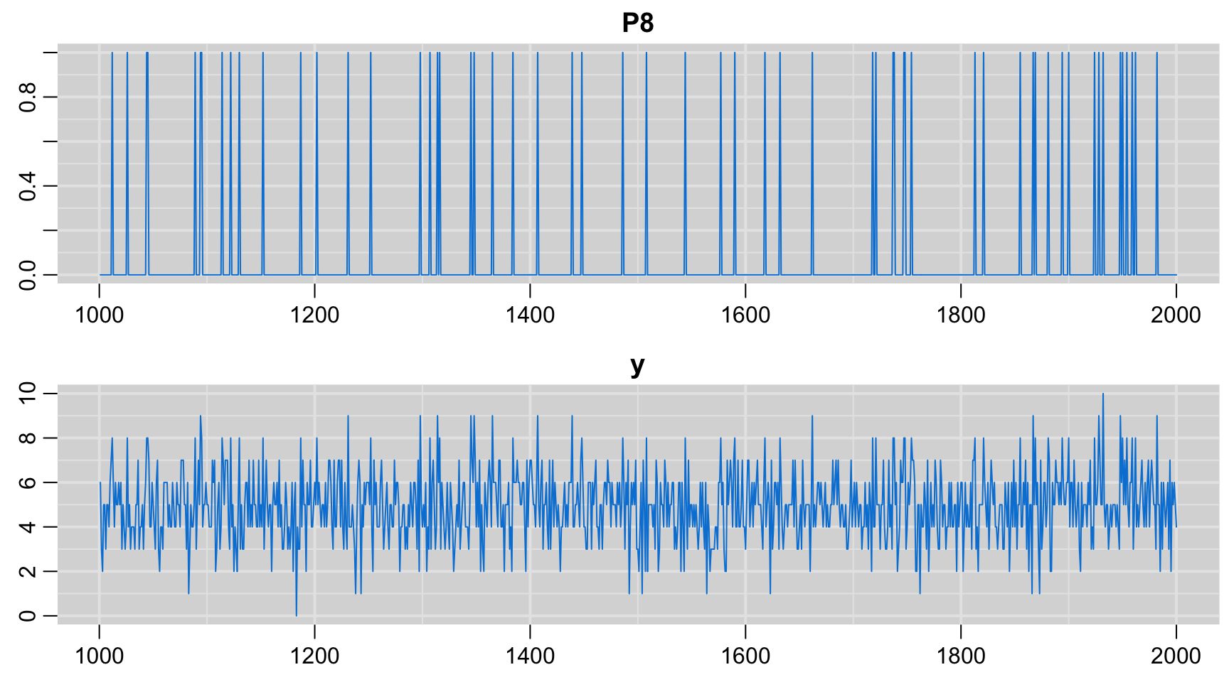
圖 96.10: History of the iterations by JAGS.
對模型進行修改,嘗試計算相同設計的試驗,在徵集了30名患者,新藥的有效率爲0.7時,15名或者以內的患者有顯著療效的事件發生的概率是多少?
model{
  y ~ dbin(0.7, 30)
  P15 <- step(15.5 - y) # = 1 if Y is 15 or fewer
}
OpenBUGS Codes:
# Step 1 check model
modelCheck(paste(bugpath, "/backupfiles/coinmodel30.txt", sep = ""))
# there is no data so just compile the model
modelCompile(numChains = 1)
# There is no need to provide initial values as this is
# a Monte Carlo forward sampling from a known distribution
# but the program still requires initial values to begin
# generate a random value.
modelGenInits() #
# Set monitors on nodes of interest#### SPECIFY, WHICH PARAMETERS TO TRACE:
parameters <- c("P15", "y")
samplesSet(parameters)
# Generate 1000 iterations
modelUpdate(10000)

#### SHOW POSTERIOR STATISTICS
sample.statistics <- samplesStats("*")
print(sample.statistics)

#### PUT THE SAMPLED VALUES IN ONE R DATA FRAME:
chain <- data.frame(P15 = samplesSample("P15"),
                    y = samplesSample("y"))
#### PLOT THE HISTOGRAMS OF THE SAMPLED VALUES
## samplesDensity("*", 1,  mfrow = c(2,2), ask=NULL)

for(p_ in parameters)
  {
    hist(chain[[p_]], main=p_,
         ylab=NA, xlab=NA, #prob = TRUE,
         nclas=50, col="red")
  }
JAGS code:
# Step 1 check model
jagsModel <- jags.model(file = paste(bugpath, "/backupfiles/coinmodel30.txt", sep = ""),
                        n.chains = 1)
## Compiling model graph
## Resolving undeclared variables
## Allocating nodes
## Graph information:
## Observed stochastic nodes: 0
## Unobserved stochastic nodes: 1
## Total graph size: 6
##
## Initializing model# Step 2 update 1000 iterations
update(jagsModel, n.iter = 1000,
progress.bar="none")
# Step 3 set monitor variables
codaSamples <- coda.samples(
jagsModel,
variable.names = c("P15", "y"),
n.iter = 10000,
progress.bar="none")
summary(codaSamples)##
## Iterations = 1001:11000
## Thinning interval = 1
## Number of chains = 1
## Sample size per chain = 10000
##
## 1. Empirical mean and standard deviation for each variable,
## plus standard error of the mean:
##
## Mean SD Naive SE Time-series SE
## P15 0.0169 0.1289 0.001289 0.001289
## y 21.0385 2.4936 0.024936 0.024936
##
## 2. Quantiles for each variable:
##
## 2.5% 25% 50% 75% 97.5%
## P15 0 0 0 0 0
## y 16 19 21 23 26#### PLOT THE HISTOGRAMS OF THE SAMPLED VALUES
ggSample <- ggs(codaSamples)
ggs_histogram(ggSample, bins = 18)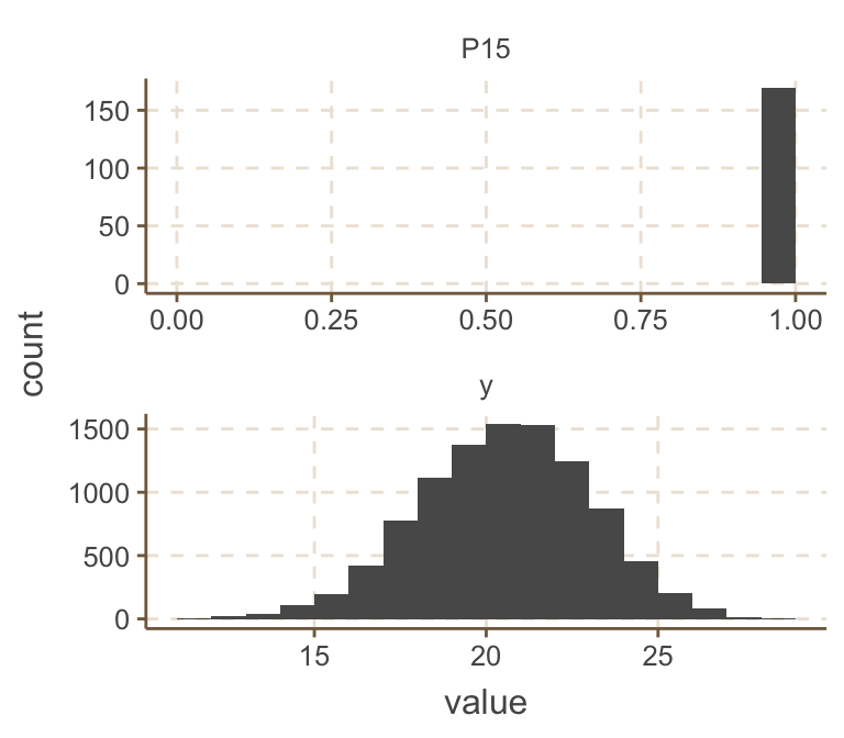
圖 96.11: Predictive distribution of the nodes of interest.
所以此時少於或等於15人得到症狀改善的事件發生的概率被推測爲1.8%。
- 藥物治療臨牀試驗
藥物臨牀試驗的例子中,我們建立的模型如下:
#  Monte Carlo predictions for Drug example

model{
    theta   ~ dbeta(9.2,13.8)          # prior distribution
    y         ~ dbin(theta,20)         # sampling distribution
    P.crit   <- step(y-14.5)           # =1 if y >= 15, 0 otherwise
}把這個模型存儲成drug-MC.txt文件之後,可以使用OpenBUGS完成該模型的蒙特卡羅模擬試驗計算:
# Step 1 check model
modelCheck(paste(bugpath, "/backupfiles/drug-MC.txt", sep = ""))
# there is no data so just compile the model
modelCompile(numChains = 1)
# There is no need to provide initial values as this is
# a Monte Carlo forward sampling from a known distribution
# but the program still requires initial values to begin
# generate a random value.
modelGenInits() #
# Set monitors on nodes of interest#### SPECIFY, WHICH PARAMETERS TO TRACE:
parameters <- c("theta", "y", "P.crit")
samplesSet(parameters)
# Generate 1000 iterations
modelUpdate(10000)

#### SHOW POSTERIOR STATISTICS
sample.statistics <- samplesStats("*")
print(sample.statistics)

#### PUT THE SAMPLED VALUES IN ONE R DATA FRAME:
chain <- data.frame(theta = samplesSample("theta"),
                    y = samplesSample("y"),
                    P.crit = samplesSample("P.crit"))
#### PLOT THE DENSITY and HISTOGRAMS OF THE SAMPLED VALUES
##1. samplesDensity("*", 1,  mfrow = c(2,2), ask=NULL)
# or 2. by looping
# for(p_ in parameters)
#   {
#     hist(chain[[p_]], main=p_,
#          ylab=NA, xlab=NA, #prob = TRUE,
#          nclas=50, col="red")
#   }
par(mfrow=c(1,2))

plot(density(chain$theta), main = "theta sample 10000",
     ylab = "P(theta)", xlab = "theta", col = "red")
hist(chain$y, main = "y sample 10000", ylab = "P(Y)",
     xlab = "y", col = "red", prob = TRUE)
也可以使用JAGS完成該模型的蒙特卡羅模擬試驗計算:
# Step 1 check model
jagsModel <- jags.model(file = paste(bugpath,
                                     "/backupfiles/drug-MC.txt", sep = ""),
                        n.chains = 1)
## Compiling model graph
## Resolving undeclared variables
## Allocating nodes
## Graph information:
## Observed stochastic nodes: 0
## Unobserved stochastic nodes: 2
## Total graph size: 8
##
## Initializing model# Step 2 update 1000 iterations
update(jagsModel, n.iter = 1000,
progress.bar="none")
# Step 3 set monitor variables
parameters <- c("theta", "y", "P.crit")
codaSamples <- coda.samples(
jagsModel,
variable.names = parameters,
n.iter = 10000,
progress.bar="none")
summary(codaSamples)##
## Iterations = 1001:11000
## Thinning interval = 1
## Number of chains = 1
## Sample size per chain = 10000
##
## 1. Empirical mean and standard deviation for each variable,
## plus standard error of the mean:
##
## Mean SD Naive SE Time-series SE
## P.crit 0.01600 0.125481 0.00125481 0.00125481
## theta 0.39975 0.099718 0.00099718 0.00099718
## y 7.99120 2.917083 0.02917083 0.02917083
##
## 2. Quantiles for each variable:
##
## 2.5% 25% 50% 75% 97.5%
## P.crit 0.00000 0.0000 0.00000 0.00000 0.00000
## theta 0.21688 0.3285 0.39698 0.46778 0.59986
## y 3.00000 6.0000 8.00000 10.00000 14.00000#### PLOT THE DENSITY and HISTOGRAMS OF THE SAMPLED VALUES
# par(mfrow=c(1,2))
#
ggSample <- ggs(codaSamples)
# ggSample %>%
# filter(Parameter == "theta") %>%
# ggs_density()
#
# ggSample %>%
# filter(Parameter == "y") %>%
# ggs_histogram(bin = 38)
par(mfrow=c(1,2))
Theta <- ggSample %>%
filter(Parameter == "theta")
Y <- ggSample %>%
filter(Parameter == "y")
plot(density(Theta$value), main = "theta sample 10000",
ylab = "P(theta)", xlab = "theta", col = "red")
hist(Y$value, main = "y sample 10000", ylab = "P(Y)",
xlab = "y", col = "red", prob = TRUE)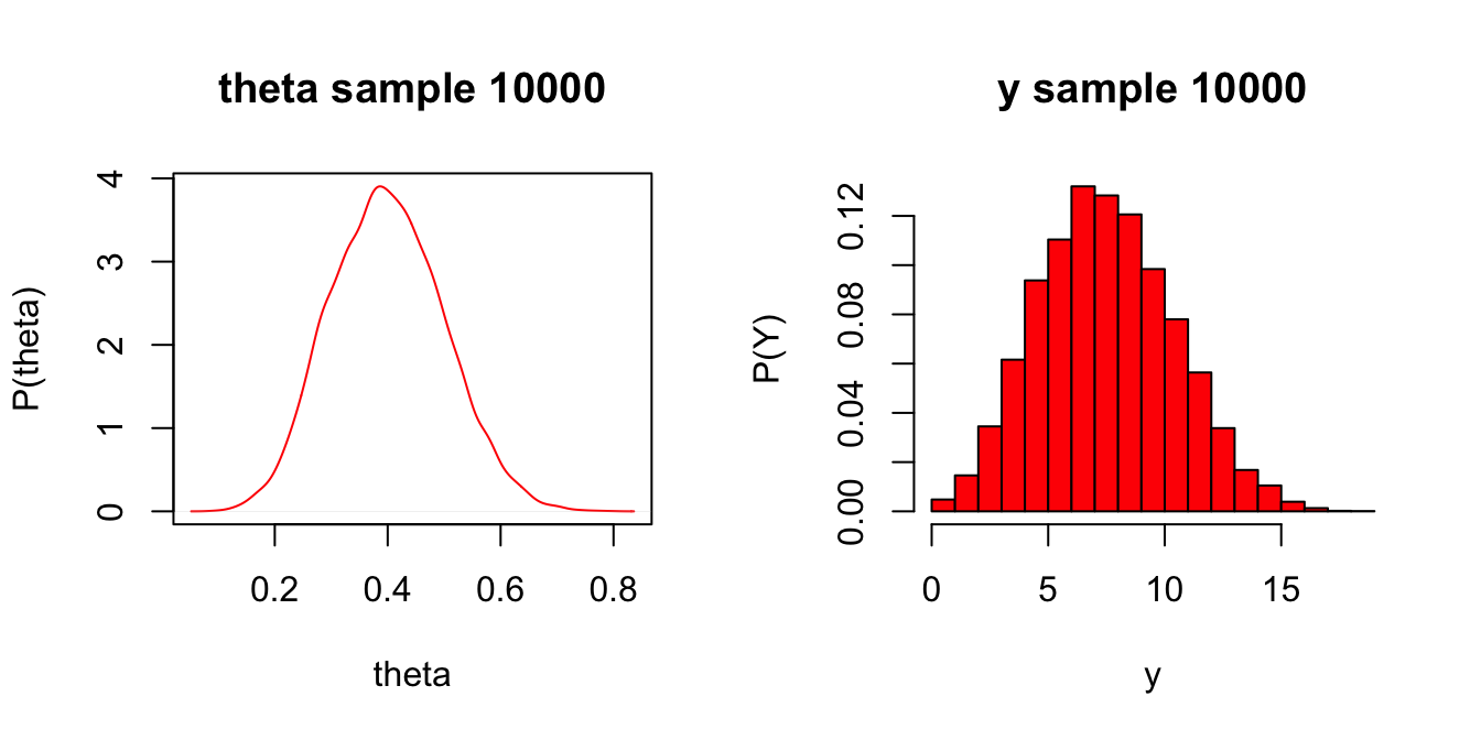
圖 96.12: Predictive distribution of the nodes of interest.
如果把藥物治療的臨牀試驗例子的先驗概率分布修改一下,修改成爲一個沒有信息的均一分布 \(\text{Uniform}(0, 1)\),模型的結果會有怎樣的變化呢?嘗試繪制成功次數的預測概率分布,此時”20名患者中大於或者等於15名患者有療效”這一事件發生的概率是多少?
#  Monte Carlo predictions for Drug example
#  with a uniform prior

model{
#   theta   ~ dbeta(9.2,13.8)          # prior distribution
  theta   ~ dunif(0,1)               # prior distribution
    y         ~ dbin(theta,20)         # sampling distribution
    P.crit   <- step(y-14.5)           # =1 if y >= 15, 0 otherwise
}
# Step 1 check model
jagsModel <- jags.model(file = paste(bugpath,
"/backupfiles/drug-MCuniform.txt", sep = ""),
n.chains = 1)## Compiling model graph
## Resolving undeclared variables
## Allocating nodes
## Graph information:
## Observed stochastic nodes: 0
## Unobserved stochastic nodes: 2
## Total graph size: 8
##
## Initializing model# Step 2 update 1000 iterations
update(jagsModel, n.iter = 1000,
progress.bar="none")
# Step 3 set monitor variables
parameters <- c("theta", "y", "P.crit")
codaSamples <- coda.samples(
jagsModel,
variable.names = parameters,
n.iter = 10000,
progress.bar="none")
summary(codaSamples)##
## Iterations = 1001:11000
## Thinning interval = 1
## Number of chains = 1
## Sample size per chain = 10000
##
## 1. Empirical mean and standard deviation for each variable,
## plus standard error of the mean:
##
## Mean SD Naive SE Time-series SE
## P.crit 0.29010 0.45383 0.0045383 0.0045383
## theta 0.50349 0.29060 0.0029060 0.0029060
## y 10.04810 6.06725 0.0606725 0.0606725
##
## 2. Quantiles for each variable:
##
## 2.5% 25% 50% 75% 97.5%
## P.crit 0.000000 0.00000 0.00000 1.00000 1.00000
## theta 0.025827 0.25146 0.50461 0.75791 0.97766
## y 0.000000 5.00000 10.00000 15.00000 20.00000#### PLOT THE DENSITY and HISTOGRAMS OF THE SAMPLED VALUES
ggSample <- ggs(codaSamples)
par(mfrow=c(1,2))
Theta <- ggSample %>%
filter(Parameter == "theta")
Y <- ggSample %>%
filter(Parameter == "y")
plot(density(Theta$value), main = "theta sample 10000",
ylab = "P(theta)", xlab = "theta", col = "red")
hist(Y$value, main = "y sample 10000", ylab = "P(Y)",
xlab = "y", col = "red", prob = TRUE)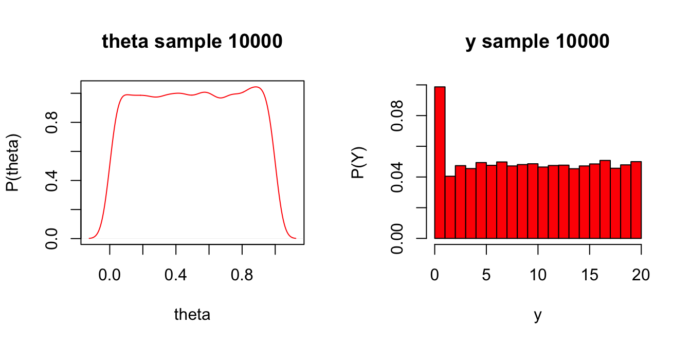
圖 96.13: Predictive distribution of the nodes of interest.
這個條件下,“20名患者中大於或者等於15名患者有療效”這一事件發生的概率爲29.2%。
- 嘗試自己來寫一個模型。
打開一個空白文檔,試着寫一個模型,它的先驗概率是一個標準正態分布,(OpenBUGS code: x ~ dnorm(0,1))。值得注意的是,在OpenBUGS的環境下,標準正態分布的描述方式和平時概率論統計學有些不一樣:概率論的標準差或者方差,在貝葉斯統計學中被冠以另一種新的概念–精確度(precision, = 1/variance)。試着嘗試用蒙特卡羅模擬試驗的方法計算標準正態分布中取值低於-1.96,和-2.326的事件發生的概率各自是多少。(已知二者的理論值分別是0.025, 0.01)。
#  Monte Carlo predictions
#  with a standard normal distribution prior

model{
  x        ~ dnorm(0, 1)             # prior distribution
    p.1     <- step(-1.96 - x)         # = 1 if x <= -1.96, 0 otherwise
    p.2     <- step(-2.32 - x)         # = 1 if x <= -2.32, 0 otherwise
}
分別對這個模型嘗試蒙特卡羅模擬試驗100, 1000, 和100000次,比較蒙特卡羅模擬試驗給出的概率估計和理論值的差異。
# Step 1 check model
jagsModel <- jags.model(file = paste(bugpath,
                                     "/backupfiles/standardnormalMC.txt", sep = ""),
                        n.chains = 1)
## Compiling model graph
## Resolving undeclared variables
## Allocating nodes
## Graph information:
## Observed stochastic nodes: 0
## Unobserved stochastic nodes: 1
## Total graph size: 11
##
## Initializing model# Step 2 update 1000 iterations
update(jagsModel, n.iter = 10,
progress.bar="none")
# Step 3 set monitor variables
parameters <- c("p.1", "p.2", "x")
codaSamples <- coda.samples(
jagsModel,
variable.names = parameters,
n.iter = 100,
progress.bar="none")
summary(codaSamples)##
## Iterations = 11:110
## Thinning interval = 1
## Number of chains = 1
## Sample size per chain = 100
##
## 1. Empirical mean and standard deviation for each variable,
## plus standard error of the mean:
##
## Mean SD Naive SE Time-series SE
## p.1 0.030000 0.17145 0.017145 0.020718
## p.2 0.020000 0.14071 0.014071 0.017909
## x 0.047827 0.95877 0.095877 0.120088
##
## 2. Quantiles for each variable:
##
## 2.5% 25% 50% 75% 97.5%
## p.1 0.0000 0.0000 0.00000 0.00000 0.5250
## p.2 0.0000 0.0000 0.00000 0.00000 0.0000
## x -2.1135 -0.5632 0.13167 0.70565 1.7822# Generate 900 iterations
codaSamples <- coda.samples(
jagsModel,
variable.names = parameters,
n.iter = 1000,
progress.bar="none")
summary(codaSamples)##
## Iterations = 111:1110
## Thinning interval = 1
## Number of chains = 1
## Sample size per chain = 1000
##
## 1. Empirical mean and standard deviation for each variable,
## plus standard error of the mean:
##
## Mean SD Naive SE Time-series SE
## p.1 0.028000 0.165055 0.0052195 0.0052195
## p.2 0.009000 0.094488 0.0029880 0.0032002
## x -0.012981 1.042048 0.0329524 0.0329524
##
## 2. Quantiles for each variable:
##
## 2.5% 25% 50% 75% 97.5%
## p.1 0.0000 0.0000 0.000000 0.00000 1.0000
## p.2 0.0000 0.0000 0.000000 0.00000 0.0000
## x -1.9831 -0.7097 -0.037555 0.69824 2.0609# Generate 100000 iterations
codaSamples <- coda.samples(
jagsModel,
variable.names = parameters,
n.iter = 100000,
progress.bar="none")
summary(codaSamples)##
## Iterations = 1111:101110
## Thinning interval = 1
## Number of chains = 1
## Sample size per chain = 100000
##
## 1. Empirical mean and standard deviation for each variable,
## plus standard error of the mean:
##
## Mean SD Naive SE Time-series SE
## p.1 0.025070 0.156339 0.00049439 0.00049439
## p.2 0.009870 0.098857 0.00031261 0.00031261
## x 0.001749 1.002820 0.00317120 0.00317120
##
## 2. Quantiles for each variable:
##
## 2.5% 25% 50% 75% 97.5%
## p.1 0.000 0.00000 0.0000000 0.00000 1.0000
## p.2 0.000 0.00000 0.0000000 0.00000 0.0000
## x -1.962 -0.67341 0.0014913 0.67986 1.9695我們知道理論上 \(x\sim N(0,1^2)\),它的均值爲0,標準差爲1。我們也能看見蒙特卡羅模擬試驗的結果,隨着我們增加其重復取樣次數二越來越接近理論值。當取樣達到十萬次以上之後,可以看到蒙特卡羅的結果已經十分之接近真實值。在一開始剛剛重復100次蒙特卡羅時,我們可以看到p.1, p.2的估計還很不準確,但是類似的,當蒙特卡羅採樣次數達到十萬次以上時,這兩個概率估計也已經十分接近真實值。另外值得注意的一點是,隨着蒙特卡羅樣本量增加,MC_error也在變得越來越小(越來越精確)。事實上,這個Naive SE本身約等於\(\frac{\text{sd}}{\sqrt{\text{sample size}}}\)。所以對\(x\)來說,經過1000次蒙特卡羅計算,\(\text{sd}(x) = 1.009\),那麼此時的Naive SE\(=\frac{1.009}{\sqrt{1000}} \approx 0.0319\),十分接近計算機給出的Naive SE = 0.03244。Naive SE本身可以作爲這個\(x\)均值的估計精確度來理解,我們同時相信,真實的理論值會落在蒙特卡羅樣本均值\(\pm 2\times\) Naive SE範圍內。
下面我們來探索一下 t分布。嘗試寫下一個BUGS模型,它的先驗概率分布是一個自由度爲4的t分布,y ~ dt(0,1,4)。然後進行10000次蒙特卡羅採樣計算,並給出概率密度分布圖。
#  Monte Carlo predictions
#  with a t distribution prior with degree of freedom = 4

model{
  y ~ dt(0, 1, 4)
}
# Step 1 check model
jagsModel <- jags.model(file = paste(bugpath,
"/backupfiles/MCt.txt", sep = ""),
n.chains = 1)## Compiling model graph
## Resolving undeclared variables
## Allocating nodes
## Graph information:
## Observed stochastic nodes: 0
## Unobserved stochastic nodes: 1
## Total graph size: 4
##
## Initializing model# Step 2 update 1000 iterations
update(jagsModel, n.iter = 10,
progress.bar="none")
# Step 3 set monitor variables
parameters <- c("y")
codaSamples <- coda.samples(
jagsModel,
variable.names = parameters,
n.iter = 10000,
progress.bar="none")
summary(codaSamples)##
## Iterations = 11:10010
## Thinning interval = 1
## Number of chains = 1
## Sample size per chain = 10000
##
## 1. Empirical mean and standard deviation for each variable,
## plus standard error of the mean:
##
## Mean SD Naive SE Time-series SE
## -0.014838 1.387851 0.013879 0.013879
##
## 2. Quantiles for each variable:
##
## 2.5% 25% 50% 75% 97.5%
## -2.758298 -0.751031 -0.023335 0.741610 2.724315#### PLOT THE DENSITY and HISTOGRAMS OF THE SAMPLED VALUES
ggSample <- ggs(codaSamples)
Y <- ggSample %>%
filter(Parameter == "y")
plot(density(Y$value), main = "y sample 10000",
ylab = "P(y)", xlab = "y", col = "red")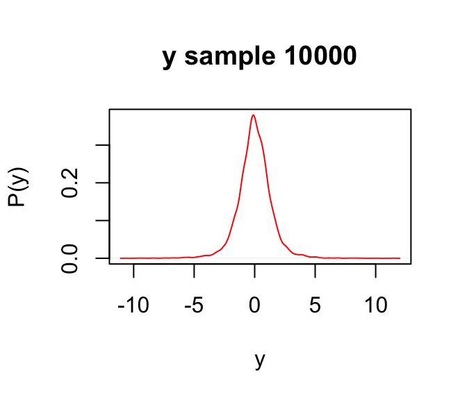
圖 96.14: Predictive distribution of the nodes of interest.
下面再嘗試計算一個來自均值爲1,標準差爲2的正態分布的隨機變量,它的三次方的期望值是多少。已知標準差\(SD = 2\),那麼方差爲\(Var = 4\),那麼翻譯成BUGS語言就是精確度爲 \(\frac{1}{4} = 0.25\)。
#  Monte Carlo predictions

model{
  y ~ dnorm(1, 0.25)
  ycubed <- pow(y, 3) # note how to write power in BUGS
}
# Step 1 check model
jagsModel <- jags.model(file = paste(bugpath,
"/backupfiles/MCcube.txt", sep = ""),
n.chains = 1)## Compiling model graph
## Resolving undeclared variables
## Allocating nodes
## Graph information:
## Observed stochastic nodes: 0
## Unobserved stochastic nodes: 1
## Total graph size: 5
##
## Initializing model# Step 2 update 1000 iterations
update(jagsModel, n.iter = 10,
progress.bar="none")
# Step 3 set monitor variables
parameters <- c("y", "ycubed")
codaSamples <- coda.samples(
jagsModel,
variable.names = parameters,
n.iter = 10000,
progress.bar="none")
summary(codaSamples)##
## Iterations = 11:10010
## Thinning interval = 1
## Number of chains = 1
## Sample size per chain = 10000
##
## 1. Empirical mean and standard deviation for each variable,
## plus standard error of the mean:
##
## Mean SD Naive SE Time-series SE
## y 1.0018 1.9908 0.019908 0.02055
## ycubed 13.0391 39.7504 0.397504 0.40482
##
## 2. Quantiles for each variable:
##
## 2.5% 25% 50% 75% 97.5%
## y -2.8439 -0.341175 1.0053 2.3391 4.9108
## ycubed -23.0013 -0.039713 1.0159 12.7975 118.4277#### PLOT THE DENSITY and HISTOGRAMS OF THE SAMPLED VALUES
ggSample <- ggs(codaSamples)
par(mfrow=c(1,2))
Y <- ggSample %>%
filter(Parameter == "y")
Ycubed <- ggSample %>%
filter(Parameter == "ycubed")
plot(density(Y$value), main = "y sample 10000",
ylab = "P(y)", xlab = "y", col = "red")
plot(density(Ycubed$value), main = "ycubed sample 100000",
ylab = "P(ycubed)", xlab = "ycubed", col = "red")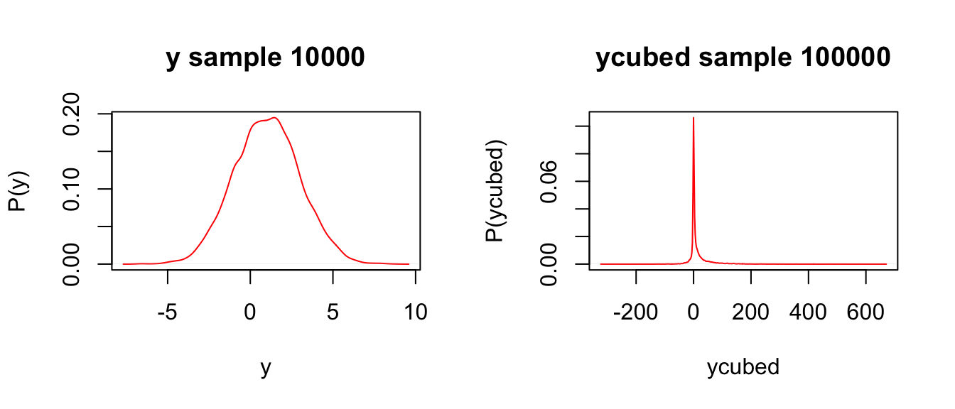
圖 96.15: Predictive distribution of the nodes of interest.
所以,一個隨機變量如果它來自一個均值爲1,標準差爲2的正態分布,那麼它的三次方的期望值是13,注意ycubed右側的尾巴很長。