第 66 章 檢查你的模型 Model Checking - GLM
每次定義一個 GLM 模型的時候 (Section 58.2),均分三步走,所以一個模型會出錯的部分,就在這三步驟中的任何一步:
- 因變量分佈定義錯誤 (或者分佈的假設不成立) mis-specified distribution: 因變量之間是否相互獨立,且服從某個已知的分佈,這兩個條件中的任意一個不能滿足,第一步都無法成立。例如,最常見的是我們用泊松迴歸模型來擬合計數型數據時,因爲缺乏一些關鍵變量,導致模型遇到過度離散的問題 (over-dispersed for a Poisson distribution due to an omitted covariate);
- 線性預測方程定義錯誤 mis-specified linear predictor: 線性預測方程中放入的變量,有的可能需要被轉換 (連續型轉換成分類型,或者是需要數學轉換)。或者是應該加入的交互作用項被我們粗心忽略了;
- 鏈接方程錯誤 mis-specified link function: 對前一步定義好的線性預測方程,第三步的鏈接方程指定很可能出現錯誤。或者是,我們可以考慮選用別的鏈接方程 (\(\text{log instead of logit}\)),改變了鏈接方程之後,很可能原先認爲有交互作用的變量之間交互作用就消失了 (Section 63.4)。
本章介紹一些廣義線性迴歸模型診斷的方法,這些手段雖然偶爾有一些檢驗方法,但更多的診斷方法需要繪圖通過視覺判斷。介紹邏輯迴歸時解釋過模型比較時使用的模型偏差 (deviance) 概念 (Section 60.3.2) Pearson 的擬合優度檢驗,以及使用 Hosmer-Lemeshow 檢驗法檢驗個人二進制變量數據的邏輯迴歸擬合優度 (Section 60.4) 法。值得注意的是,這些方法是一種整體檢驗 (global test),其零假設是 “模型可以擬合數據”,如果擬合優度檢驗的結果是拒絕這個零假設,那麼可以認爲模型建立的不佳,即接受 “模型不能擬合數據” 的替代假設。如果擬合優度檢驗的結果是無法拒絕零假設,那麼我們僅僅只能認爲無證據證明 “模型不可以擬合數據”,而不能證明設計的模型可以良好的擬合數據。所以,擬合優度的檢驗結果可以警告我們模型擬合有沒有錯誤,卻不能證明這個模型到底是不是一個良好的模型 (個人感覺應把擬合優度檢驗 goodness of fit 的名稱改爲 擬合劣度檢驗 badness of fit)。
66.1 線性預測方程的定義
線性預測方程定義錯誤的最常見的就是“忽略了不該忽略的交互作用”,及連續型變量可能被以不恰當的方式加入預測方程中。當然,你可以通過把一個變量放入模型前後,該變量本身的迴歸係數是否有意義 (Wald test) 或者你關心的預測變量的迴歸係數的變化程度 (magnitude of the corresponding parameter estimate) 來判斷是否保留這個變量在你的模型裏。這麼做的時候,你要當心自己陷入多重比較 (multiple testing) 的陷阱 (某次或者某幾次出現的統計學有意義的結果,可以僅僅是由於偶然,而不是因爲它真的有意義)。
66.1.1 殘差
觀測值跟擬合值之間的差距,就是我們常說的殘差。
以二項分佈數據爲例,
\[Y_i\sim\text{Bin}(n_i, \pi_i), \\ \text{where n is the number of subjects in one group} \\ \text{logit}(\pi_i) = \eta_i\]
其第 \(i\) 個觀測值的原始殘差 (raw residual),是
\[ \begin{aligned} r_i & = y_i - \hat\mu_i \\ & = y_i - n_i\hat\pi_i \end{aligned} \]
觀測值 \(Y_i\) 的變化程度 (variability) 本身並不是一成不變的 (會根據模型中加入的共變量而改變),其變化程度可能是觀測值 \(Y_i\) 的方差導致的。二項分佈數據的方差已知是 \(\text{Var}(Y_i) = n_i\pi_i(1-\pi_i)\)。舉個栗子,如果 \(n_i = 10, \hat\pi_i = 0.01, Y_i = 10\),那麼 \(r_i \approx 10\),這是一個很差的擬合效果。如果,\(n_i = 100000, \hat\pi_i = 0.5, Y_i = 5010\),那麼 \(r_i = 10\),此時的殘差也是 \(10\) 又證明了這是一個擬合效果良好的模型。相同的殘差,由於方差不同,判斷則不一樣,所以我們需要有一個類似簡單線性迴歸中標準化殘差 (Section 32.6.1) 的過程 – Pearson 殘差:
\[ p_i = \frac{r_i}{\sqrt{\hat{\text{Var}}}(Y_i)} \]
所以,二項分佈數據的 Pearson 殘差公式爲
\[ p_i = \frac{r_i}{\sqrt{n_i\hat\pi_i(1-\hat\pi_i)}} \]
Pearson 殘差的平方和,就是 Pearson 卡方統計量,在只有分類變量的邏輯迴歸模型中可以用於擬合度診斷 (Section 67.1),自由度爲 \(1\):
\[ \sum_i^Np^2_i = \text{Pearson's } \chi^2 \text{ statistic} \]
和標準化 Pearson 殘差相似地,另一個選項是使用偏差殘差 (deviance residual)。只要使偏差殘差 \(d_i\) 和原始殘差 \(r_i\) 保持相同的符號,偏差殘差也可以被標準化用於模型診斷。
用二項分佈數據的例子,
\[ \begin{aligned} d_i & = \text{sign}(r_i)\sqrt{2\{ y_i\text{ln}(\frac{y_i}{\hat\mu_i}) + (n_i - y_i)\text{ln}(\frac{n_i-y_i}{n_i - \hat\mu_i})\}} \\ \sum_{i=1}^n d^2 = D & = 2\sum_{i=1}^N\{ y_i\text{ln}(\frac{y_i}{\hat\mu_i}) + (n_i - y_i)\text{ln}(\frac{n_i - y_i}{n_i - \hat\mu_i}) \} \end{aligned} \]
66.4 NHANES 飲酒量數據實例
數據的變量和每個變量的解釋如下表,總樣本量是 2548 人,飲酒量大於 5 杯每日者被定義爲重度飲酒者。
| Variable | Description |
|---|---|
gender |
1=male, 2=female |
ageyrs |
Age in years at survey |
bmi |
Body mass index \((\text{kg/m}^2)\) |
sbp |
Systolic blood pressure \((\text{mmHg})\) |
ALQ130 |
Reported average number of drinks per day |
NHANES <- read_dta("../backupfiles/nhanesglm.dta")
NHANES <- NHANES %>%
  mutate(Gender = ifelse(gender == 1, "Male", "Female")) %>%
    mutate(Gender = factor(Gender, levels = c("Male", "Female")))
with(NHANES, table(gender))
## gender
## 1 2
## 1391 1157NHANES <- mutate(NHANES, Heavydrinker = ALQ130 > 5)
Model_NH <- glm(Heavydrinker ~ gender + ageyrs, data = NHANES, family = binomial(link = "logit"))
logistic.display(Model_NH);summary(Model_NH)##
## Logistic regression predicting Heavydrinker
##
## crude OR(95%CI) adj. OR(95%CI) P(Wald's test) P(LR-test)
## gender (cont. var.) 0.17 (0.12,0.24) 0.16 (0.11,0.23) < 0.001 < 0.001
##
## ageyrs (cont. var.) 0.97 (0.97,0.98) 0.97 (0.96,0.98) < 0.001 < 0.001
##
## Log-likelihood = -801.292
## No. of observations = 2548
## AIC value = 1608.5839##
## Call:
## glm(formula = Heavydrinker ~ gender + ageyrs, family = binomial(link = "logit"),
## data = NHANES)
##
## Deviance Residuals:
## Min 1Q Median 3Q Max
## -0.86408 -0.57154 -0.34828 -0.22281 2.85177
##
## Coefficients:
## Estimate Std. Error z value Pr(>|z|)
## (Intercept) 1.6410885 0.2755315 5.9561 2.584e-09 ***
## gender -1.8249474 0.1736041 -10.5121 < 2.2e-16 ***
## ageyrs -0.0304506 0.0039882 -7.6351 2.257e-14 ***
## ---
## Signif. codes: 0 '***' 0.001 '**' 0.01 '*' 0.05 '.' 0.1 ' ' 1
##
## (Dispersion parameter for binomial family taken to be 1)
##
## Null deviance: 1810.21 on 2547 degrees of freedom
## Residual deviance: 1602.58 on 2545 degrees of freedom
## AIC: 1608.58
##
## Number of Fisher Scoring iterations: 6當用邏輯迴歸模型擬合數據,線性迴歸方程加入年齡和性別時,數據給出了極強的證據證明性別和年齡和是否爲重度飲酒者都有很大的關係。但是,擬合完這樣一個邏輯迴歸模型之後,我們最大的擔心是,模型中的年齡變量和 \(\text{logit}(\text{P}(Y=1))\) 之間的關係,用簡單線性是不是恰當?要檢驗這樣的擔憂,最好的方法是追加一個非線性轉換後的年齡值,去看看模型的擬合程度是否得到改善:
NHANES <- mutate(NHANES, age2 = ageyrs^2)
Model_NH2 <- glm(Heavydrinker ~ gender + ageyrs + age2, data = NHANES, family = binomial(link = "logit"))
logistic.display(Model_NH2) ; summary(Model_NH2)
##
## Logistic regression predicting Heavydrinker
##
## crude OR(95%CI) adj. OR(95%CI) P(Wald's test) P(LR-test)
## gender (cont. var.) 0.17 (0.12,0.24) 0.16 (0.11,0.23) < 0.001 < 0.001
##
## ageyrs (cont. var.) 0.9726 (0.9652,0.9801) 1.01 (0.966,1.056) 0.663 0.662
##
## age2 (cont. var.) 0.9997 (0.9996,0.9998) 0.9996 (0.9991,1) 0.073 0.067
##
## Log-likelihood = -799.6124
## No. of observations = 2548
## AIC value = 1607.2249##
## Call:
## glm(formula = Heavydrinker ~ gender + ageyrs + age2, family = binomial(link = "logit"),
## data = NHANES)
##
## Deviance Residuals:
## Min 1Q Median 3Q Max
## -0.80207 -0.60342 -0.32980 -0.23312 2.87272
##
## Coefficients:
## Estimate Std. Error z value Pr(>|z|)
## (Intercept) 0.83418082 0.52440600 1.5907 0.11167
## gender -1.82748612 0.17346142 -10.5354 < 2e-16 ***
## ageyrs 0.00991164 0.02272523 0.4362 0.66273
## age2 -0.00043512 0.00024311 -1.7898 0.07348 .
## ---
## Signif. codes: 0 '***' 0.001 '**' 0.01 '*' 0.05 '.' 0.1 ' ' 1
##
## (Dispersion parameter for binomial family taken to be 1)
##
## Null deviance: 1810.21 on 2547 degrees of freedom
## Residual deviance: 1599.22 on 2544 degrees of freedom
## AIC: 1607.22
##
## Number of Fisher Scoring iterations: 6擬合了年齡的平方 (age2) 進入邏輯迴歸模型中之後,age2 的迴歸係數的 Wald 檢驗結果是 \(p = 0.073\),這證明用簡單的線性關係把年齡放在模型裏並不算不妥當 (not unreasonable)。
另外,可以提取 Model_NH 的標準化 Pearson 殘差和年齡作如下的散點圖:
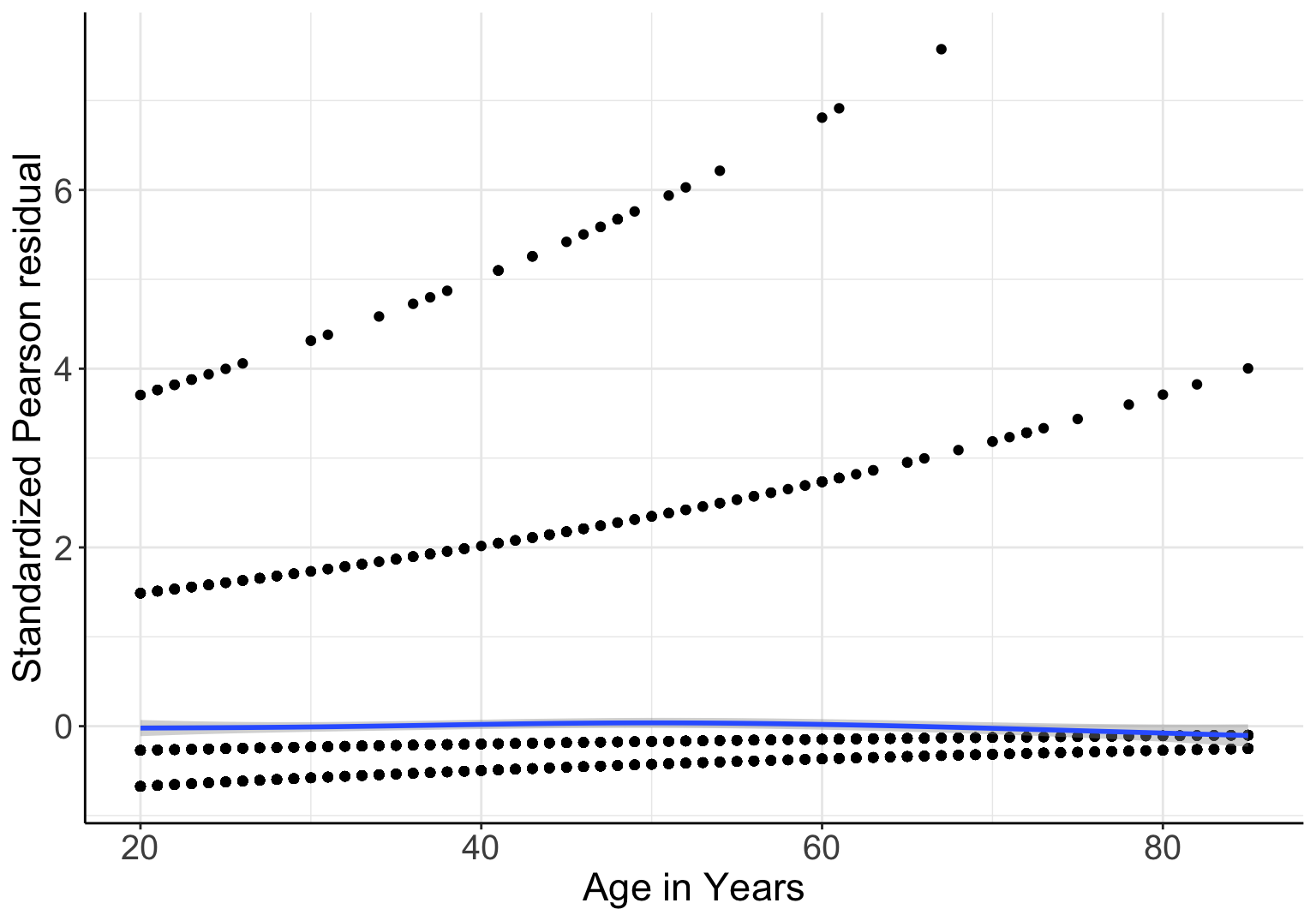
圖 66.1: Standardized Pearson residuals agianst age, in logistic model with gender and linear age as covariates
圖 66.1 中靠近橫軸的藍色實線是 LOWESS 平滑曲線,它十分接近平直的橫線,也證明了 Pearson 標準化殘差值和年齡本身並無關聯。這同時也佐證了,將年齡以連續型共變量的形式放入本次邏輯迴歸模型中並非不合理 (not unreasonable)。
下一步,我們再來考慮,模型中加入 bmi 是否合理 (能改善模型的擬合度):
Model_NH3 <- glm(Heavydrinker ~ gender + ageyrs + bmi, data = NHANES, family = binomial(link = "logit"))
logistic.display(Model_NH3) ; summary(Model_NH3)
##
## Logistic regression predicting Heavydrinker
##
## crude OR(95%CI) adj. OR(95%CI) P(Wald's test) P(LR-test)
## gender (cont. var.) 0.17 (0.12,0.24) 0.16 (0.11,0.23) < 0.001 < 0.001
##
## ageyrs (cont. var.) 0.97 (0.97,0.98) 0.97 (0.96,0.98) < 0.001 < 0.001
##
## bmi (cont. var.) 0.9965 (0.9756,1.0179) 1.0084 (0.9855,1.0318) 0.477 0.479
##
## Log-likelihood = -801.0412
## No. of observations = 2548
## AIC value = 1610.0825##
## Call:
## glm(formula = Heavydrinker ~ gender + ageyrs + bmi, family = binomial(link = "logit"),
## data = NHANES)
##
## Deviance Residuals:
## Min 1Q Median 3Q Max
## -0.93712 -0.57479 -0.34466 -0.22359 2.82847
##
## Coefficients:
## Estimate Std. Error z value Pr(>|z|)
## (Intercept) 1.4251178 0.4096026 3.4793 0.0005028 ***
## gender -1.8299784 0.1738183 -10.5281 < 2.2e-16 ***
## ageyrs -0.0306880 0.0040105 -7.6518 1.982e-14 ***
## bmi 0.0083460 0.0117336 0.7113 0.4769053
## ---
## Signif. codes: 0 '***' 0.001 '**' 0.01 '*' 0.05 '.' 0.1 ' ' 1
##
## (Dispersion parameter for binomial family taken to be 1)
##
## Null deviance: 1810.21 on 2547 degrees of freedom
## Residual deviance: 1602.08 on 2544 degrees of freedom
## AIC: 1610.08
##
## Number of Fisher Scoring iterations: 6BMI的迴歸係數是否爲零的 Wald 檢驗 \(p=0.477\),提示數據無法提供證據去反對零假設:“調整了年齡和性別之後,BMI 和是否是重度飲酒者的概率的對數比值 \(\text{log-odds}\) 之間無線性關係”,也就是二者之間可能有非線性關係。如果把 Pearson 標準化殘差和 BMI 作殘差散點圖,如下所示:
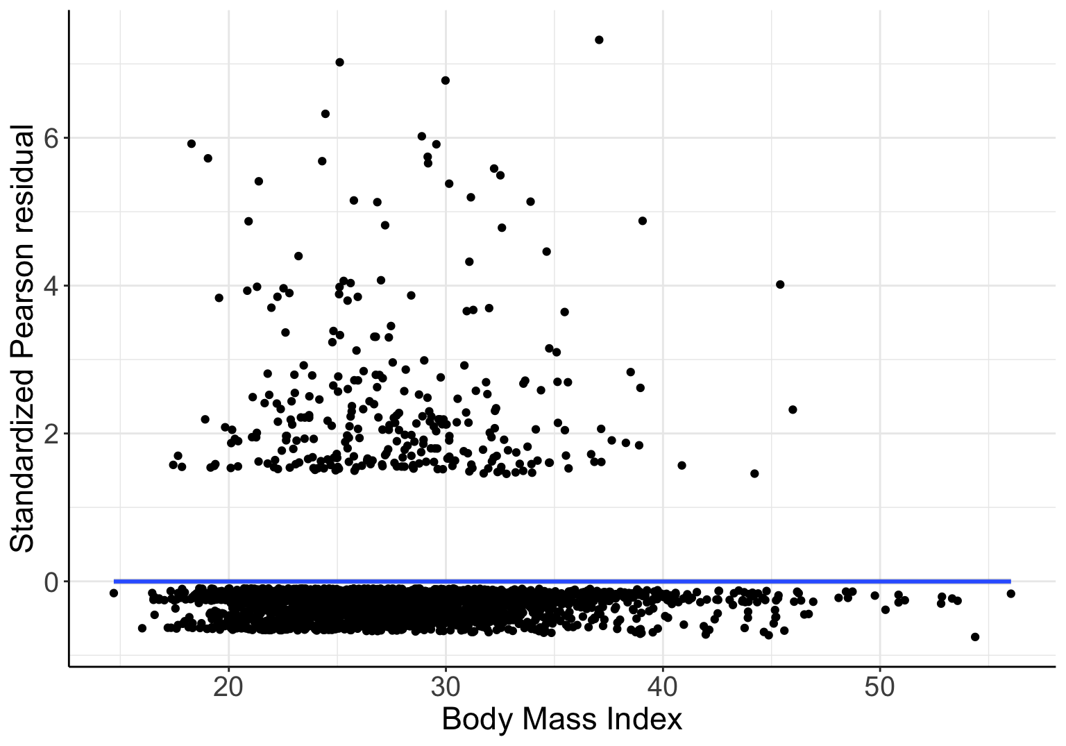
圖 66.2: Standardized Pearson residuals agianst BMI, in logistic model with gender and linear age as covariates
此殘差圖 66.2 的 LOWESS 平滑曲線卻提示我們,BMI 和殘差之間不完全是毫無關係的 (應該是非線性的,拋物線關係?)。如果我們把 BMI 取平方放入模型中再看其結果:
NHANES <- mutate(NHANES, bmi2 = bmi^2)
Model_NH4 <- glm(Heavydrinker ~ gender + ageyrs + bmi + bmi2, data = NHANES, family = binomial(link = "logit"))
summary(Model_NH4)
##
## Call:
## glm(formula = Heavydrinker ~ gender + ageyrs + bmi + bmi2, family = binomial(link = "logit"),
## data = NHANES)
##
## Deviance Residuals:
## Min 1Q Median 3Q Max
## -0.93349 -0.57566 -0.34335 -0.21636 2.85524
##
## Coefficients:
## Estimate Std. Error z value Pr(>|z|)
## (Intercept) -2.1277529 1.4806329 -1.4371 0.15070
## gender -1.7784430 0.1745978 -10.1859 < 2.2e-16 ***
## ageyrs -0.0323786 0.0040936 -7.9096 2.583e-15 ***
## bmi 0.2551992 0.1003287 2.5436 0.01097 *
## bmi2 -0.0041230 0.0016854 -2.4464 0.01443 *
## ---
## Signif. codes: 0 '***' 0.001 '**' 0.01 '*' 0.05 '.' 0.1 ' ' 1
##
## (Dispersion parameter for binomial family taken to be 1)
##
## Null deviance: 1810.21 on 2547 degrees of freedom
## Residual deviance: 1594.91 on 2543 degrees of freedom
## AIC: 1604.91
##
## Number of Fisher Scoring iterations: 6##
## Logistic regression predicting Heavydrinker
##
## crude OR(95%CI) adj. OR(95%CI) P(Wald's test) P(LR-test)
## gender (cont. var.) 0.17 (0.12,0.24) 0.17 (0.12,0.24) < 0.001 < 0.001
##
## ageyrs (cont. var.) 0.97 (0.97,0.98) 0.97 (0.96,0.98) < 0.001 < 0.001
##
## bmi (cont. var.) 1 (0.98,1.02) 1.29 (1.06,1.57) 0.011 0.006
##
## bmi2 (cont. var.) 0.9999 (0.9995,1.0002) 0.9959 (0.9926,0.9992) 0.014 0.007
##
## Log-likelihood = -797.4554
## No. of observations = 2548
## AIC value = 1604.9108## Likelihood ratio test
##
## Model 1: Heavydrinker ~ gender + ageyrs
## Model 2: Heavydrinker ~ gender + ageyrs + bmi + bmi2
## #Df LogLik Df Chisq Pr(>Chisq)
## 1 3 -801.292
## 2 5 -797.455 2 7.67309 0.021568 *
## ---
## Signif. codes: 0 '***' 0.001 '**' 0.01 '*' 0.05 '.' 0.1 ' ' 1通過似然比檢驗比較加了 bmi, bmi2 兩個共變量的模型和只有 gender, ageyrs 兩個共變量的模型 \((p=0.022)\),提示我們 BMI 和是否是重度飲酒者 (概率的對數比值 \(\text{log-odds}\)) 之間的關係並非簡單的線性關係。不過這樣的關係似乎並不是特別的明顯,圖 66.2 的平滑曲線的彎曲程度也沒有特別明顯。所以,在這樣的情況下,有的統計學家可能還是會選擇不放 BMI 進入模型裏。
66.5 Practical 10
繼續沿用 NHANES 數據,此次練習我們把重點放在收集到的收縮期血壓數據上。定義收縮期血壓大於 140 \(\text{mmHg}\) 者爲高血壓患者。
# 1. load the data and define a binary variable indicating whether
#    each observation has hypertension (1) or not (0)
NHANES <- read_dta("../backupfiles/nhanesglm.dta")
NHANES <- NHANES %>%
  mutate(Gender = ifelse(gender == 1, "Male", "Female")) %>%
    mutate(Gender = factor(Gender, levels = c("Male", "Female")))
NHANES <- mutate(NHANES, hypertension = sbp >= 140)
tab1(NHANES$hypertension, graph = FALSE)
## NHANES$hypertension :
## Frequency Percent Cum. percent
## FALSE 2116 83 83
## TRUE 432 17 100
## Total 2548 100 100# 2. Bearing in mind that we know blood pressure increases with age
# we begin by including age into a logistic regression for the
# the binary hypertension variable. We can use a lowess smoother
# plot to examine how the probability of hypertension varies with
# age.
pi <- with(NHANES, predict(loess(hypertension ~ ageyrs)))
with(NHANES, scatter.smooth(ageyrs, logit(pi), pch = 20, span = 0.6, lpars =
list(col = "blue", lwd = 3, lty = 1), col=rgb(0,0,0,0.004),
xlab = "Age in years",
ylab = "Logit(probability) of Hypertension",
frame = FALSE))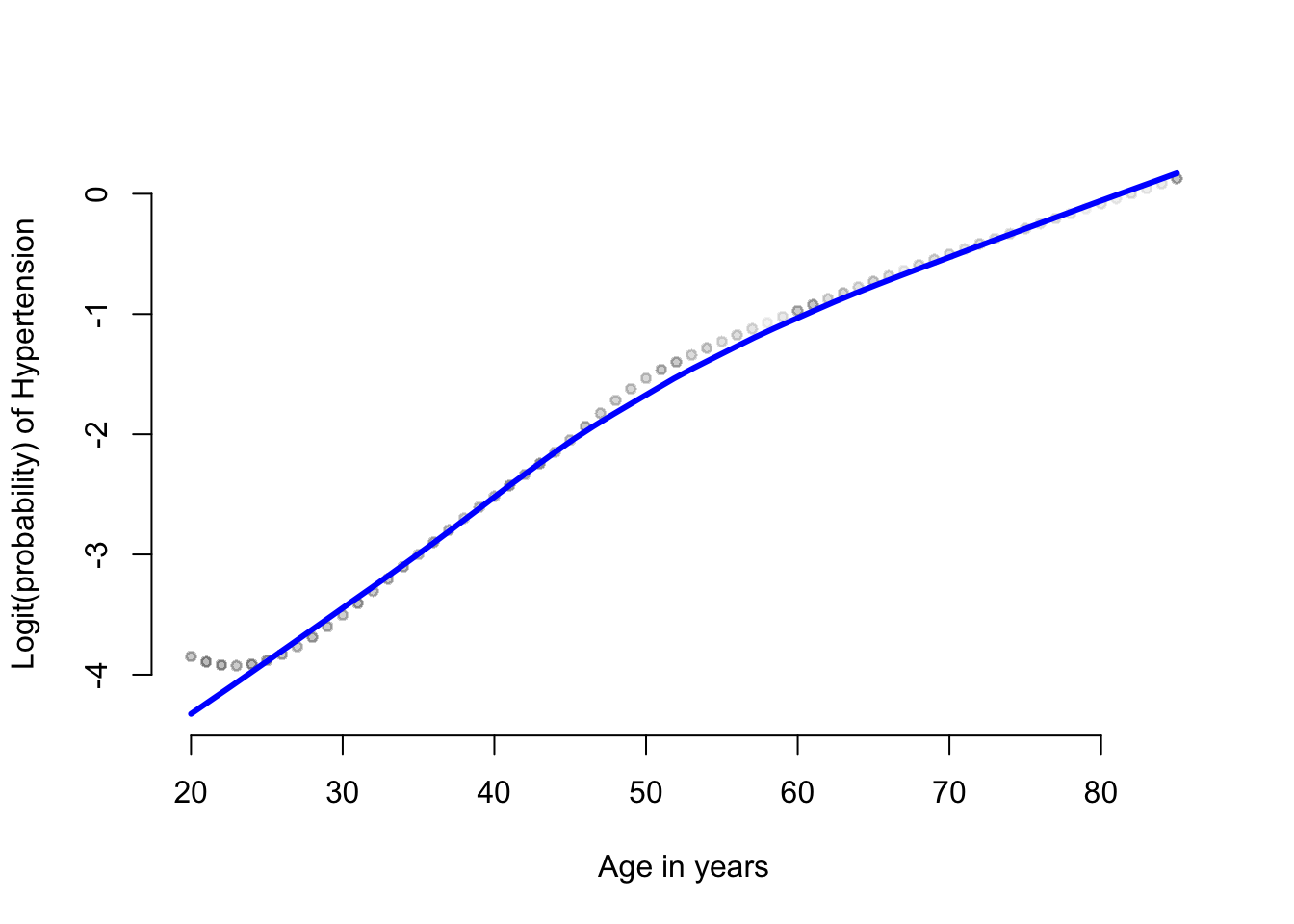
圖 66.3: The loess plot of the observed proportin with hypertension against age. Span = 0.6
Lowess 平滑曲線圖提示,高血壓患病的可能性的 \(\text{logit}\),和年齡之間的關係似乎不是簡單直線關係。我們可能需要把年齡本身和年齡的平方放入邏輯迴歸模型中去看看。
# 3. Include age into the logistic regression in the way suggested by the lowess plot.
#    do your results support your findings from the previous graph?
NHANES <- mutate(NHANES, agesq = ageyrs^2)
Model_NH5 <- glm(hypertension ~ ageyrs + agesq, data = NHANES, family = binomial(link = "logit"))
logistic.display(Model_NH5) ; summary(Model_NH5)
##
## Logistic regression predicting hypertension
##
## crude OR(95%CI) adj. OR(95%CI) P(Wald's test) P(LR-test)
## ageyrs (cont. var.) 1.07 (1.06,1.07) 1.15 (1.1,1.21) < 0.001 < 0.001
##
## agesq (cont. var.) 1.0005 (1.0005,1.0006) 0.9993 (0.9989,0.9997) 0.001 < 0.001
##
## Log-likelihood = -943.7811
## No. of observations = 2548
## AIC value = 1893.5622##
## Call:
## glm(formula = hypertension ~ ageyrs + agesq, family = binomial(link = "logit"),
## data = NHANES)
##
## Deviance Residuals:
## Min 1Q Median 3Q Max
## -1.20772 -0.61574 -0.33152 -0.18319 2.97415
##
## Coefficients:
## Estimate Std. Error z value Pr(>|z|)
## (Intercept) -6.92931228 0.67205641 -10.311 < 2.2e-16 ***
## ageyrs 0.13933661 0.02419897 5.758 8.514e-09 ***
## agesq -0.00067035 0.00020870 -3.212 0.001318 **
## ---
## Signif. codes: 0 '***' 0.001 '**' 0.01 '*' 0.05 '.' 0.1 ' ' 1
##
## (Dispersion parameter for binomial family taken to be 1)
##
## Null deviance: 2319.51 on 2547 degrees of freedom
## Residual deviance: 1887.56 on 2545 degrees of freedom
## AIC: 1893.56
##
## Number of Fisher Scoring iterations: 6正如同 Lowess 平滑曲線建議的那樣,數據提供了極強的證據證明年齡和患有高血壓概率的對數比值 \((\text{log-odds})\) 之間呈現的是拋物線關係。
# 4. Generate Pearson residuals and investigate whether the way in
#    which you have included age in the logistic regression in the
#    previous part is correct.

# obtain the standardized Pearson residuals by covariate pattern
Diag <- LogisticDx::dx(Model_NH5)
ggplot(Diag, aes(x = ageyrs, y = sPr)) +  geom_point() +
  geom_smooth(span = 0.9, se = FALSE) +  theme_bw()  +
  theme(axis.text = element_text(size = 15),
  axis.text.x = element_text(size = 15),
  axis.text.y = element_text(size = 15)) +
  labs(x = "Age in years", y = "standardised Pearson residual")  +
  theme(axis.title = element_text(size = 17), axis.text = element_text(size = 8),
        axis.line = element_line(colour = "black"),
    panel.border = element_blank(),
    panel.background = element_blank())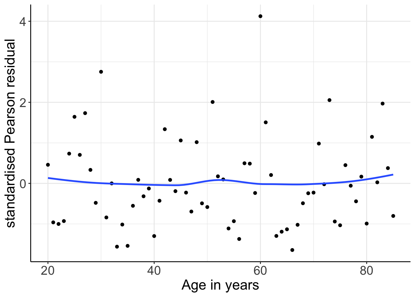
圖 66.4: Standardized Pearson residuals (by covariate pattern) vs. age. Logistic mdoel with linear and quadratic age as covariates.
標準化 Pearson 殘差 (共變量模式) 和年齡之間的散點圖 66.4 提示此時的殘差和年齡之間再無明顯的關係。也就是說,年齡作爲連續變量和高血壓患病概率的對數比值之間的關係,用拋物線 (二次方程) 擬合並非不合理 (not unreasonable)。
# 5. Next, use individual level residuals to examine whether BMI ought to be
#    included in the model, and depending on what you find, continue with you
#    previous model or add BMI. In the latter case, generate new residuals and
#    assess if you have included BMI using the most appropriate functional form.
NHANES$stresPearson <- boot::glm.diag(Model_NH5)$rp
ggplot(NHANES, aes(x = bmi, y = stresPearson)) +
  geom_point() +
  theme_bw() +
  geom_smooth(span = 0.8, se = FALSE) +
  theme(axis.text = element_text(size = 15),
  axis.text.x = element_text(size = 15),
  axis.text.y = element_text(size = 15)) +
  labs(x = "Body Mass Index", y = "Standardized Pearson residual")  +
  theme(axis.title = element_text(size = 17), axis.text = element_text(size = 8),
        axis.line = element_line(colour = "black"),
    panel.border = element_blank(),
    panel.background = element_blank())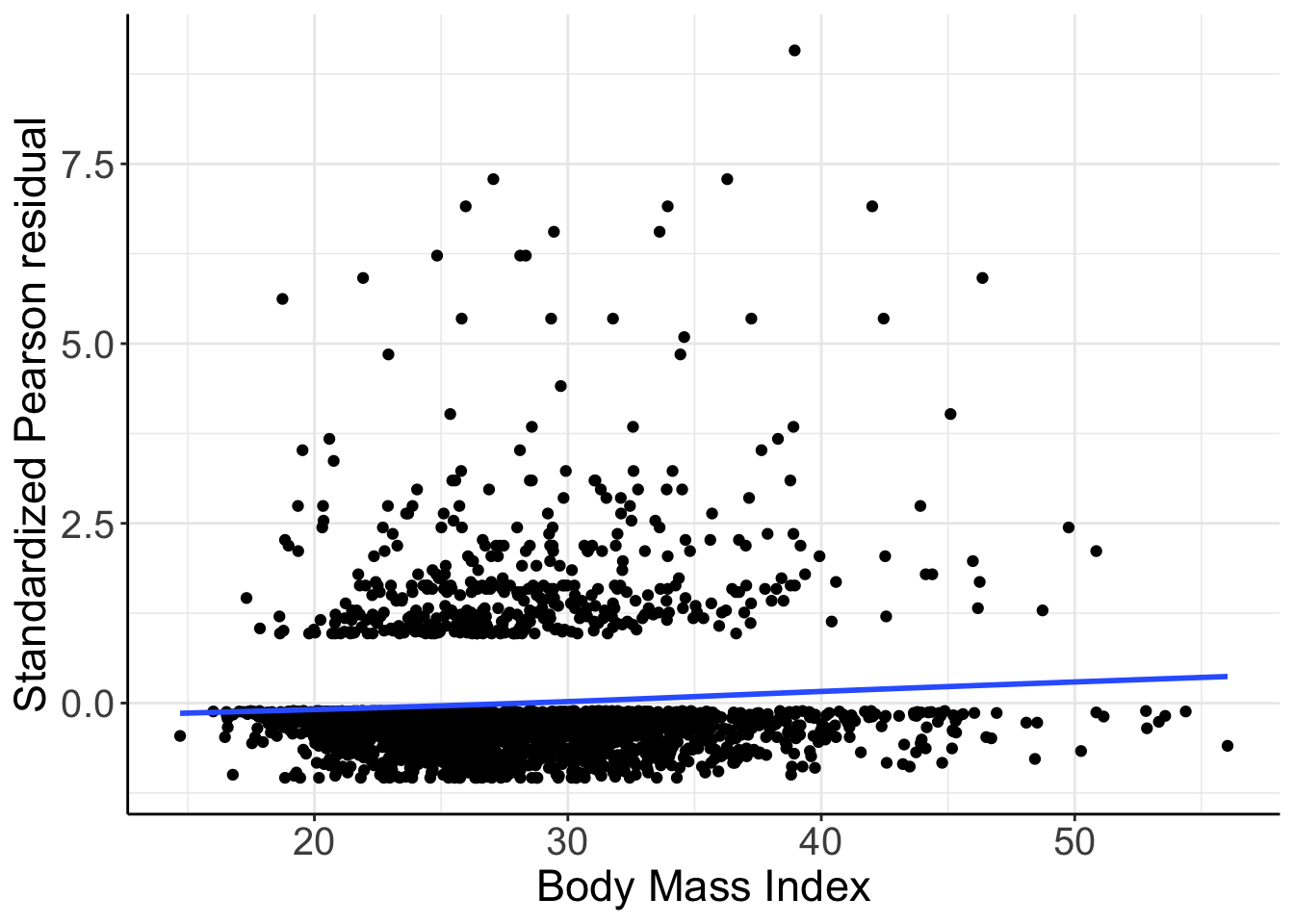
圖 66.5: Standardized Pearson residuals vs. BMI. Logistic mdoel with just linear and quadratic age as covariates.
圖 66.5,提示,標準化 Pearson 殘差和連續型 BMI 值之間應該存在相關性,也就是該圖提示需要加入連續型變量 BMI 進入邏輯迴歸模型中去!
Model_NH6 <- glm(hypertension ~ ageyrs + agesq + bmi, data = NHANES, family = binomial(link = "logit"))
logistic.display(Model_NH6) ; summary(Model_NH6)
##
## Logistic regression predicting hypertension
##
## crude OR(95%CI) adj. OR(95%CI) P(Wald's test) P(LR-test)
## ageyrs (cont. var.) 1.07 (1.06,1.07) 1.14 (1.09,1.2) < 0.001 < 0.001
##
## agesq (cont. var.) 1.0005 (1.0005,1.0006) 0.9994 (0.999,0.9998) 0.005 0.004
##
## bmi (cont. var.) 1.02 (1.01,1.04) 1.03 (1.01,1.05) 0.007 0.007
##
## Log-likelihood = -940.1583
## No. of observations = 2548
## AIC value = 1888.3166##
## Call:
## glm(formula = hypertension ~ ageyrs + agesq + bmi, family = binomial(link = "logit"),
## data = NHANES)
##
## Deviance Residuals:
## Min 1Q Median 3Q Max
## -1.32095 -0.61276 -0.33033 -0.18260 2.85207
##
## Coefficients:
## Estimate Std. Error z value Pr(>|z|)
## (Intercept) -7.54111034 0.71010300 -10.6197 < 2.2e-16 ***
## ageyrs 0.13107997 0.02430813 5.3924 6.951e-08 ***
## agesq -0.00059168 0.00021030 -2.8135 0.004900 **
## bmi 0.02840320 0.01046359 2.7145 0.006638 **
## ---
## Signif. codes: 0 '***' 0.001 '**' 0.01 '*' 0.05 '.' 0.1 ' ' 1
##
## (Dispersion parameter for binomial family taken to be 1)
##
## Null deviance: 2319.51 on 2547 degrees of freedom
## Residual deviance: 1880.32 on 2544 degrees of freedom
## AIC: 1888.32
##
## Number of Fisher Scoring iterations: 6加入連續型變量 BMI 進入模型後,bmi 項的 Wald 檢驗結果果然證實了 之前殘差圖提示的 BMI 和高血壓患病概率之間存在相關性。再對 Model_NH6 的殘差和 bmi 作殘差散點圖:
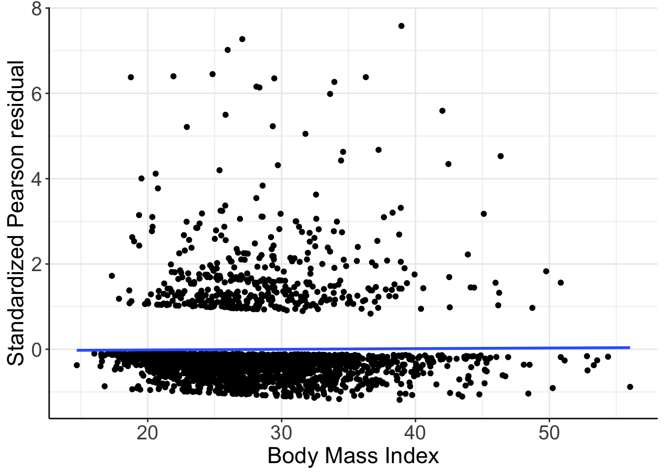
圖 66.6: Standardized Pearson residuals vs. BMI. Logistic mdoel with linear and quadratic age and BMI as covariates.
現在的殘差散點圖提示殘差和 bmi 之間不再有關係,所以之前把 bmi 加入邏輯迴歸模型是個並非不合理 (not unreasonable)的選擇。
# 6. So far we have ingored gender. Explore whether gender should be included
#    in the model. including whether or not the other covariates included
#    already interact with gender with their effects on hypertension.
Model_NH7 <- glm(hypertension ~ ageyrs + agesq + bmi + Gender,
                 data = NHANES, family = binomial(link = "logit"))
logistic.display(Model_NH7) ; summary(Model_NH7)
##
## Logistic regression predicting hypertension
##
## crude OR(95%CI) adj. OR(95%CI) P(Wald's test) P(LR-test)
## ageyrs (cont. var.) 1.07 (1.06,1.07) 1.14 (1.09,1.2) < 0.001 < 0.001
##
## agesq (cont. var.) 1.0005 (1.0005,1.0006) 0.9994 (0.999,0.9998) 0.005 0.004
##
## bmi (cont. var.) 1.02 (1.01,1.04) 1.03 (1.01,1.05) 0.009 0.009
##
## Gender: Female vs Male 1.1 (0.9,1.36) 1.24 (0.98,1.56) 0.07 0.07
##
## Log-likelihood = -938.5164
## No. of observations = 2548
## AIC value = 1887.0328##
## Call:
## glm(formula = hypertension ~ ageyrs + agesq + bmi + Gender, family = binomial(link = "logit"),
## data = NHANES)
##
## Deviance Residuals:
## Min 1Q Median 3Q Max
## -1.37006 -0.61503 -0.33044 -0.18099 2.89593
##
## Coefficients:
## Estimate Std. Error z value Pr(>|z|)
## (Intercept) -7.64411420 0.71405324 -10.7052 < 2.2e-16 ***
## ageyrs 0.13206361 0.02435967 5.4214 5.913e-08 ***
## agesq -0.00059709 0.00021066 -2.8344 0.004592 **
## bmi 0.02730943 0.01043204 2.6178 0.008849 **
## GenderFemale 0.21213190 0.11703954 1.8125 0.069912 .
## ---
## Signif. codes: 0 '***' 0.001 '**' 0.01 '*' 0.05 '.' 0.1 ' ' 1
##
## (Dispersion parameter for binomial family taken to be 1)
##
## Null deviance: 2319.51 on 2547 degrees of freedom
## Residual deviance: 1877.03 on 2543 degrees of freedom
## AIC: 1887.03
##
## Number of Fisher Scoring iterations: 6## Likelihood ratio test
##
## Model 1: hypertension ~ ageyrs + agesq + bmi
## Model 2: hypertension ~ ageyrs + agesq + bmi + Gender
## #Df LogLik Df Chisq Pr(>Chisq)
## 1 4 -940.158
## 2 5 -938.516 1 3.28378 0.069967 .
## ---
## Signif. codes: 0 '***' 0.001 '**' 0.01 '*' 0.05 '.' 0.1 ' ' 1# some evidence of an effect of gender.
# the Wald test and the likelihood ratio test are both borderline
# statistically significant.
Model_NH8 <- glm(hypertension ~ ageyrs + agesq + bmi*Gender,
data = NHANES, family = binomial(link = "logit"))
logistic.display(Model_NH8)##
## Logistic regression predicting hypertension
##
## crude OR(95%CI) adj. OR(95%CI) P(Wald's test) P(LR-test)
## ageyrs (cont. var.) 1.07 (1.06,1.07) 1.14 (1.09,1.2) < 0.001 < 0.001
##
## agesq (cont. var.) 1.0005 (1.0005,1.0006) 0.9994 (0.999,0.9998) 0.006 0.005
##
## bmi (cont. var.) 1.02 (1.01,1.04) 1.05 (1.01,1.08) 0.005 < 0.001
##
## Gender: Female vs Male 1.1 (0.9,1.36) 3.01 (0.9,10) 0.072 0.072
##
## bmi:GenderFemale - 0.97 (0.93,1.01) 0.139 0.139
##
## Log-likelihood = -937.423
## No. of observations = 2548
## AIC value = 1886.846## Likelihood ratio test
##
## Model 1: hypertension ~ ageyrs + agesq + bmi + Gender
## Model 2: hypertension ~ ageyrs + agesq + bmi * Gender
## #Df LogLik Df Chisq Pr(>Chisq)
## 1 5 -938.516
## 2 6 -937.423 1 2.18675 0.1392# no strong evidence of an interaction between BMI and gender
# from both wald test and likelihood ratio test.
Model_NH9 <- glm(hypertension ~ ageyrs*Gender + agesq + bmi,
data = NHANES, family = binomial(link = "logit"))
logistic.display(Model_NH9)##
## Logistic regression predicting hypertension
##
## crude OR(95%CI) adj. OR(95%CI) P(Wald's test) P(LR-test)
## ageyrs (cont. var.) 1.07 (1.06,1.07) 1.13 (1.08,1.19) < 0.001 < 0.001
##
## Gender: Female vs Male 1.1 (0.9,1.36) 0.34 (0.14,0.84) 0.02 0.018
##
## agesq (cont. var.) 1.0005 (1.0005,1.0006) 0.9994 (0.999,0.9998) 0.004 0.003
##
## bmi (cont. var.) 1.02 (1.01,1.04) 1.03 (1.01,1.05) 0.008 0.009
##
## ageyrs:GenderFemale - 1.02 (1.01,1.04) 0.004 0.004
##
## Log-likelihood = -934.2658
## No. of observations = 2548
## AIC value = 1880.5315## Likelihood ratio test
##
## Model 1: hypertension ~ ageyrs + agesq + bmi + Gender
## Model 2: hypertension ~ ageyrs * Gender + agesq + bmi
## #Df LogLik Df Chisq Pr(>Chisq)
## 1 5 -938.516
## 2 6 -934.266 1 8.50127 0.003549 **
## ---
## Signif. codes: 0 '***' 0.001 '**' 0.01 '*' 0.05 '.' 0.1 ' ' 1## Likelihood ratio test
##
## Model 1: hypertension ~ ageyrs + agesq + bmi
## Model 2: hypertension ~ ageyrs * Gender + agesq + bmi
## #Df LogLik Df Chisq Pr(>Chisq)
## 1 4 -940.158
## 2 6 -934.266 2 11.7851 0.00276 **
## ---
## Signif. codes: 0 '***' 0.001 '**' 0.01 '*' 0.05 '.' 0.1 ' ' 1增加性別項進入邏輯迴歸模型以後,數據提供了臨界有意義證據 \((p = 0.070)\) 證明了調整了年齡和 BMI 以後,高血壓的患病概率依然和性別有關係。增加了 BMI 和性別的交互作用項之後發現,無證據證明性別和 BMI 之間存在有意義的交互作用 \((p=0.139)\)。但是,增加了年齡和性別的交互作用項以後,發現了有很強的證據證明性別和年齡之間存在交互作用 \((p=0.004)\)。增加性別以及性別和年齡的交互作用項,顯著提升了模型對數據的擬合度 \((p = 0.0028)\)。此處,我們可以下結論認爲,雖然加入年齡本身,對模型擬合程度提升有有限的幫助,但是當模型考慮了年齡和性別的交互作用之後,擬合數據的程度得到極爲顯著的改善。
當然,想要繼續下去也是可以的,例如 Model_NH9 的前提下,再加入年齡平方與性別的交互作用項,會發現其 Wald 檢驗結果提示年齡平方,和性別的交互作用是沒有意義的 \((p=0.58)\)。
# 7. Based on your final model, calculate fitted probabilities for an individual
#    aged 60 years, at BMI values from 20 to 40 in increments of 5, separately
#    for men and women, and plot the resulting values.

a <- data.frame(bmi = seq(20, 40, 5), ageyrs = rep(60, 5), agesq = rep(3600, 5), Gender = factor(rep("Male", 5)))
b <- data.frame(bmi = seq(20, 40, 5), ageyrs = rep(60, 5), agesq = rep(3600, 5), Gender = factor(rep("Female", 5)))

Predict_men <- predict(Model_NH9, a, se.fit = TRUE)$fit
Predict_men_se <- predict(Model_NH9, a, se.fit = TRUE)$se.fit
Point_pred_men <- exp(Predict_men)/(1+exp(Predict_men))
PredictCI_men_L <- exp(Predict_men - 1.96*Predict_men_se)/(1+exp(Predict_men- 1.96*Predict_men_se))
PredictCI_men_U <- exp(Predict_men + 1.96*Predict_men_se)/(1+exp(Predict_men+ 1.96*Predict_men_se))
cbind(Point_pred_men, PredictCI_men_L, PredictCI_men_U)
## Point_pred_men PredictCI_men_L PredictCI_men_U
## 1 0.20999989 0.16990237 0.25663492
## 2 0.23409879 0.19980473 0.27227618
## 3 0.26005285 0.22575914 0.29755387
## 4 0.28780311 0.24411252 0.33583907
## 5 0.31724500 0.25701542 0.38428866Predict_women <- predict(Model_NH9, b, se.fit = TRUE)$fit
Predict_women_se <- predict(Model_NH9, b, se.fit = TRUE)$se.fit
Point_pred_women <- exp(Predict_women)/(1+exp(Predict_women))
PredictCI_women_L <- exp(Predict_women - 1.96*Predict_women_se)/(1+exp(Predict_women- 1.96*Predict_women_se))
PredictCI_women_U <- exp(Predict_women + 1.96*Predict_women_se)/(1+exp(Predict_women+ 1.96*Predict_women_se))
cbind(Point_pred_women, PredictCI_women_L, PredictCI_women_U)## Point_pred_women PredictCI_women_L PredictCI_women_U
## 1 0.24913421 0.20076523 0.30471354
## 2 0.27615418 0.23478059 0.32175308
## 3 0.30491460 0.26477267 0.34825967
## 4 0.33528289 0.28659479 0.38774675
## 5 0.36707847 0.30191960 0.43748678