第 75 章 隨機回歸系數模型 random coefficient model
這一章節我們把隨機截距模型進一步擴展,在隨機效應部分增加隨機斜率成分 (random slope)。這樣的模型又稱隨機系數模型 (random coefficient model) 或 隨機斜率模型 (random slope model)。
75.1 GCSE scores 實例
第一章介紹過的 65 所中學學生在入學前的閱讀水平成績和畢業時的考試成績的 GCSE 數據,用來作爲本章介紹概念的實例。我們先對其中學校編號爲 1 的學生做兩個成績的線性回歸:
gcse_selected <- read_dta("../backupfiles/gcse_selected.dta")
M_sch1 <- lm(gcse ~ lrt, data = gcse_selected[gcse_selected$school == 1, ])

summary(M_sch1)
##
## Call:
## lm(formula = gcse ~ lrt, data = gcse_selected[gcse_selected$school ==
## 1, ])
##
## Residuals:
## Min 1Q Median 3Q Max
## -22.4876 -5.4427 -1.0177 6.1932 15.4687
##
## Coefficients:
## Estimate Std. Error t value Pr(>|t|)
## (Intercept) 3.833302 0.982238 3.9026 0.0002141 ***
## lrt 0.709341 0.092006 7.7097 5.771e-11 ***
## ---
## Signif. codes: 0 '***' 0.001 '**' 0.01 '*' 0.05 '.' 0.1 ' ' 1
##
## Residual standard error: 8.29 on 71 degrees of freedom
## Multiple R-squared: 0.45569, Adjusted R-squared: 0.44802
## F-statistic: 59.44 on 1 and 71 DF, p-value: 5.7708e-11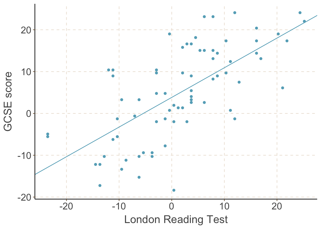
圖 75.1: GCSE versus LRT in school 1
當我們重復同樣的實驗,給 65 所學校 (48號學校除外,它只有兩個學生) 一一繪制回歸直線的時候,你得到的一簇直線是這樣紙的:
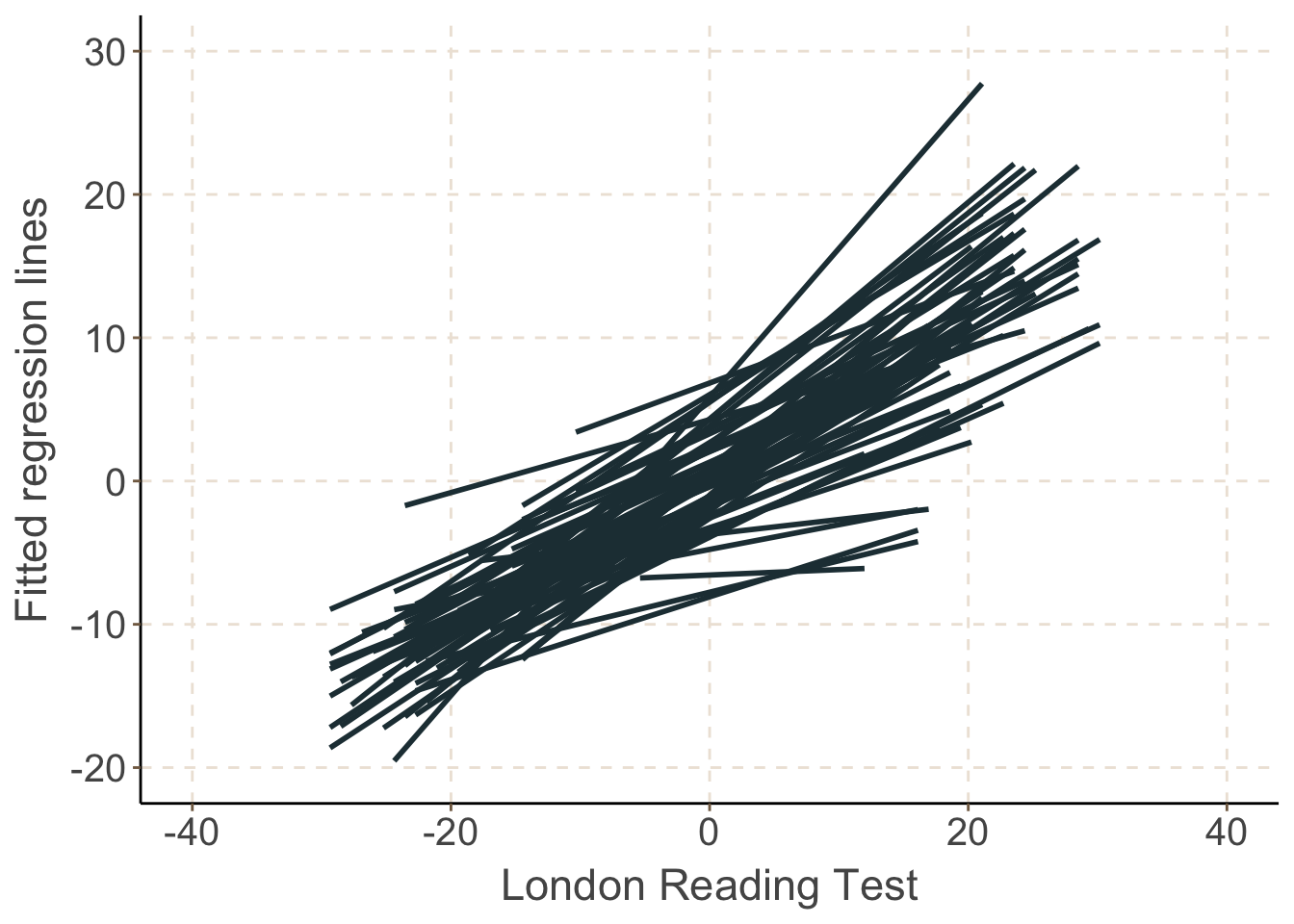
圖 75.2: Predicted regression lines of GCSE versus LRT scores: separate estimates from each school
實際上這麼多學校學生的成績前後回歸線,其截距和斜率各不相同 (圖75.2)。這些斜率和截距的總結歸納如下:
##
## No. of observations = 64
##
##   Var. name   obs. mean   median  s.d.   min.   max.
## 1 (Intercept) 64   -0.18  -0.33   3.29   -8.52  6.84
## 2 lrt         64   0.54   0.54    0.18   0.04   1.08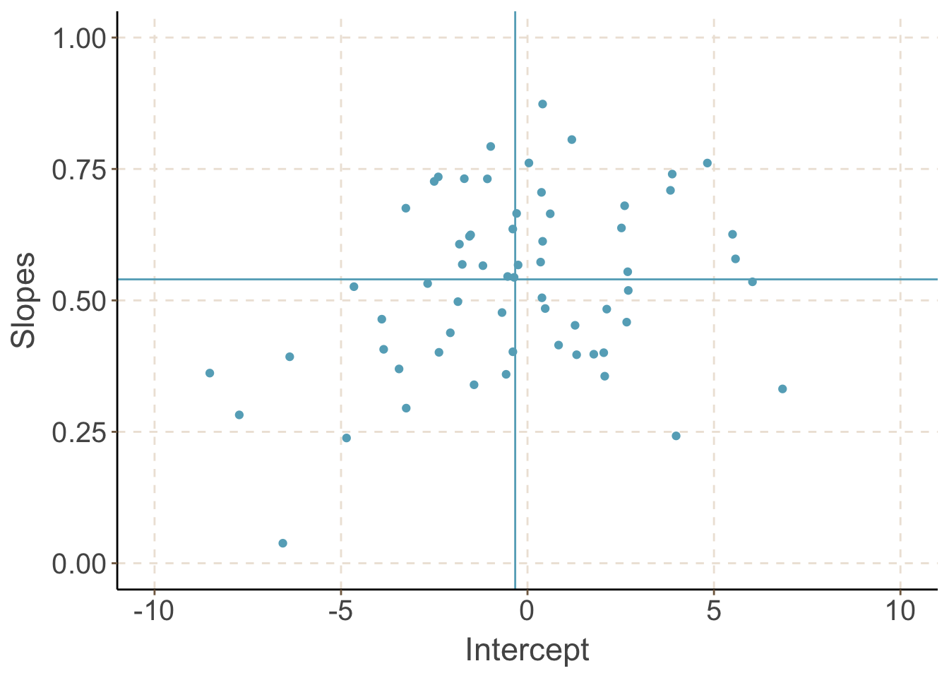
圖 75.3: School specific slopes and intercepts
圖 75.3 展示的是這些回歸直線各自的截距 (x 軸) 和斜率 (y 軸) 的散點圖。縱橫添加的兩條直線分別是截距和斜率的均值的位置。很明顯,截距和斜率之間本身是呈現正相關的 (相關系數 0.36): 如果一個學校學生入學時成績一般,但是畢業時 GCSE 成績較高,說明那所學校本身對學生成績的提升作用明顯。
經過擬合64個線性回歸模型,獲得 \(64\times3\) 個不同的回歸線的參數 (截距,斜率,和殘差方差)。所以我們可以提出的關於 “學校” 這個個體,它們各自的入學前後成績作出的回歸線獲得的三個參數,在它的 “人羣 (可以是英國國內的中學,全歐洲的中學,或者是全世界的中學)” 中是隨機分布在一些 “均值” 附近的。
75.2 隨機回歸系數的實質
在隨機截距模型中,截距可以隨機分布在某個均值周圍,但是每條回歸直線我們默認其解釋變量和結果變量之間的關系是一樣的 (相同斜率的一簇直線)。現在,我們來把這個模型擴展,放寬它對斜率的限制,允許不同的層與層之間不僅僅可以有不同的截距,還可以有不同的斜率:
\[ \begin{equation} Y_{ij} = (\beta_0 + u_{0j}) + (\beta_1 + u_{1j})X_{1ij} + e_{ij} \end{equation} \tag{75.1} \]
其中:
- \(u_{0j}:\) 是隨機截距成分 (第 \(j\) 層數據和總體均值 \(\beta_0\) 之間的差異)
- \(u_{1j}:\) 是隨機斜率成分 (第 \(j\) 層數據和總體寫率 \(\beta_1\) 之間的差異)
- \(\text{E}(u_{0j}|X_{1ij}) = 0\)
- \(\text{E}(u_{1j}|X_{1ij}) = 0\)
- \(\text{E}(e_{ij}|X_{1ij},u_{0j}, u_{1j}) = 0\)
- \(u_0, u_1 \perp X_{1ij}\) (兩個隨機部分和解釋變量之間獨立不相關)
- \(u_0, u_1 \perp e_{ij}\) (兩個隨機部分和總體的隨機誤差獨立不相關)
另外,\(\mathbf{u}_j = \{u_0, u_1\}\) 服從分布:
\[ \mathbf{u}_j | X_{1ij} \sim N(\mathbf{0}, \mathbf{\sum}_{\mathbf{u}}) \]
其中的 \(\mathbf{\sum}_{\mathbf{u}}\) 是一個 \(2\times2\) 的方差協方差矩陣:
\[ \begin{aligned} \text{Where } \mathbf{u}_j & = (u_{0j}, u_{1j})^T \\ \mathbf{0} & = (0, 0)^T \\ \mathbf{\sum}_{\mathbf{u}} & =\left( \begin{array}{cc} \sigma^2_{u_{00}} & \sigma_{u_{01}} \\ \sigma_{u_{01}} & \sigma^2_{u_{11}} \\ \end{array} \right) \end{aligned} \]
\(e_{ij}\) 則服從下列分布:
\[ e_{ij} | X_{1ij}, u_{0j}, u_{1j} \sim N(0, \sigma^2_e) \]
75.3 繼續 GCSE scores 實例
繼續用 GCSE 數據,去除掉 48 號學校以後,擬合一個固定效應模型 (相同斜率,但是不同的固定截距):
FIX_inter <- lm(gcse ~ 0 + lrt + factor(school), data = gcse_selected[gcse_selected$school != 48, ])Call:
lm(formula = gcse ~ 0 + lrt + factor(school), data = gcse_selected[gcse_selected$school !=
48, ])
Residuals:
Min 1Q Median 3Q Max
-28.32 -4.77 0.22 5.08 24.41
Coefficients:
Estimate Std. Error t value Pr(>|t|)
lrt 0.5595 0.0125 44.63 < 2e-16 ***
factor(school)1 4.0823 0.8806 4.64 3.7e-06 ***
factor(school)2 5.6202 1.0154 5.53 3.3e-08 ***
................... ............
................... <Output ommited> ............
................... ............
factor(school)62 -0.5566 0.8929 -0.62 0.53306
factor(school)63 6.4827 1.3734 4.72 2.4e-06 ***
factor(school)64 1.0089 0.9808 1.03 0.30368
factor(school)65 -1.7701 0.8415 -2.10 0.03547 *
---
Signif. codes: 0 ‘***’ 0.001 ‘**’ 0.01 ‘*’ 0.05 ‘.’ 0.1 ‘ ’ 1
Residual standard error: 7.52 on 3992 degrees of freedom
Multiple R-squared: 0.442, Adjusted R-squared: 0.433
F-statistic: 48.7 on 65 and 3992 DF, p-value: <2e-16該固定效應模型 (簡單線性回歸模型) 估計的共同斜率是 0.56 (se = 0.01),和 64 個不同的固定斜率。這些固定斜率的範圍是 -9,63 到 7.91,均值是 0.03,標準差是 3.38。估計的殘差標準差是 Residual standard error: 7.52。
如果用相同的數據,我們允許截距發生隨機變動的話 (隨機截距模型):
MIX_inter <- lmer(gcse ~ lrt + (1 | school), data = gcse_selected[gcse_selected$school != 48, ], REML = TRUE)
summary(MIX_inter)
## Linear mixed model fit by REML. t-tests use Satterthwaite's method ['lmerModLmerTest']
## Formula: gcse ~ lrt + (1 | school)
## Data: gcse_selected[gcse_selected$school != 48, ]
##
## REML criterion at convergence: 28044.1
##
## Scaled residuals:
## Min 1Q Median 3Q Max
## -3.71619 -0.63094 0.02920 0.68478 3.26661
##
## Random effects:
## Groups Name Variance Std.Dev.
## school (Intercept) 9.4273 3.0704
## Residual 56.6047 7.5236
## Number of obs: 4057, groups: school, 64
##
## Fixed effects:
## Estimate Std. Error df t value Pr(>|t|)
## (Intercept) 0.031006 0.405263 59.922917 0.0765 0.9393
## lrt 0.563268 0.012471 4048.045047 45.1676 <2e-16 ***
## ---
## Signif. codes: 0 '***' 0.001 '**' 0.01 '*' 0.05 '.' 0.1 ' ' 1
##
## Correlation of Fixed Effects:
## (Intr)
## lrt 0.007隨機截距模型估計的共同斜率還是不變 (0.56, se = 0.01),總體平均截距是 0.03 (無統計學意義)。截距的 (正態) 分布的標準差是 3.07。殘差標準差,和剛才簡單現行回歸計算的殘差標準差是一樣的 (=7.52)。幾乎所有我們關心的參數估計,都接近簡單線性回歸的結果,但是隨機截距模型使用的參數個數只有 4 個,固定效應模型則用到了 66 個 (很顯然隨機截距模型更加高效)。
接下來,我們進一步擬合本章的重點模型 – 隨機參數模型:
MIX_coef <- lmer(gcse ~ lrt + (lrt | school), data = gcse_selected[gcse_selected$school != 48, ], REML = TRUE)
summary(MIX_coef)
## Linear mixed model fit by REML. t-tests use Satterthwaite's method ['lmerModLmerTest']
## Formula: gcse ~ lrt + (lrt | school)
## Data: gcse_selected[gcse_selected$school != 48, ]
##
## REML criterion at convergence: 28003
##
## Scaled residuals:
## Min 1Q Median 3Q Max
## -3.83178 -0.63196 0.03375 0.68334 3.45515
##
## Random effects:
## Groups Name Variance Std.Dev. Corr
## school (Intercept) 9.249786 3.04135
## lrt 0.014955 0.12229 0.494
## Residual 55.382877 7.44197
## Number of obs: 4057, groups: school, 64
##
## Fixed effects:
## Estimate Std. Error df t value Pr(>|t|)
## (Intercept) -0.109203 0.402635 59.913502 -0.2712 0.7872
## lrt 0.556603 0.020112 56.329985 27.6754 <2e-16 ***
## ---
## Signif. codes: 0 '***' 0.001 '**' 0.01 '*' 0.05 '.' 0.1 ' ' 1
##
## Correlation of Fixed Effects:
## (Intr)
## lrt 0.365
## optimizer (nloptwrap) convergence code: 0 (OK)
## Model failed to converge with max|grad| = 0.00420817 (tol = 0.002, component 1)這個模型,不僅允許了隨機的截距,還允許每個直線的斜率成爲隨機的斜率。此時的總體平均截距被估計爲 -0.11 (依然沒有統計學意義),標準差略微變小 (3.07 變成了 3.04)。總體平均斜率是 0.56,現在也被允許有變動,其標準差是 0.12。此時這些許許多多的估計回歸方程中,斜率和截距的相關系數是 0.49,這十分接近我們在一開始的簡單回歸64次計算獲得的斜率和截距的相關系數 (0.36)。此隨機系數模型的殘差標準差變成了 7.44,略微小於之前的 7.52。這三個模型的結果總結如下表:
| Parameter | est | se | est | se | est | se |
|---|---|---|---|---|---|---|
| \(Fixed\; part\) | ||||||
| \(\beta_0\) | -0.03 |
|
0.031 | 0.405 | -0.109 | 0.403 |
| \(\beta_1\) | 0.56 | 0.013 | 0.563 | 0.013 | 0.557 | 0.020 |
| \(Random\; part\) | ||||||
| \(\sigma_{u_{00}}\) | 3.38 |
|
3.07 | 0.312 | 3.041 | 0.311 |
| \(\sigma_{u_{11}}\) |
|
|
|
|
0.122 | 0.019 |
| \(\text{Corr}(0,1)\) |
|
|
|
|
0.494 | 0.149 |
| \(\sigma_e\) | 7.522 |
|
7.524 | 0.084 | 7.442 | 0.084 |
75.4 使用模型結果推斷
接下來,我們討論如何比較隨機系數模型,隨機截距模型,也就是如何選擇一個更優的模型。如果只是比較相同數據下,隨機系數模型和隨機截距模型的優劣,那麼只需要同時檢驗 \(u_{1j} = 0; \text{Cov}(u_{0j}, u_{1j}) = 0\)。
就用剛剛擬合好的 MIX_inter 和 MIX_coef 來比較:
MIX_coef <- lme(fixed = gcse ~ lrt, random =  ~ lrt | school, data = gcse_selected[gcse_selected$school != 48, ], method = "REML")
MIX_inter <- lme(fixed = gcse ~ lrt, random = ~ 1 | school, data = gcse_selected[gcse_selected$school != 48, ], method = "REML")

anova(MIX_inter, MIX_coef)
## Model df AIC BIC logLik Test L.Ratio p-value
## MIX_inter 1 4 28052.050 28077.281 -14022.025
## MIX_coef 2 6 28014.963 28052.809 -14001.482 1 vs 2 41.087068 <.0001值得注意的是,這裏計算的 似然比的檢驗統計量服從的是一個 自由度爲 2 的卡方分布和一個 自由度爲 1 的卡方分布的混合分布。所以報告中給出的 p 值是一個保守估計,正確的 p 值可以這樣計算:
likelihood <- as.numeric(-2*(logLik(MIX_inter) - logLik(MIX_coef)))
0.5*(1-pchisq(as.numeric(likelihood), df = 1)) + 0.5*(1-pchisq(as.numeric(likelihood), df = 2))
## [1] 6.7124639e-10另一個重要的問題是該如何去真正理解這裏隨機系數模型給出的結果呢?
該模型的結果說,“人羣”中的總體均值是 -0.11,總體斜率是 0.56 (se = 0.02, 95%CI: 0.52, 0.60)。這裏的”人羣”指的是全英國/或者全世界這樣的學校。學校水平的截距和斜率服從以這兩個數字爲均值,標準差分別是 3.04 和 0.12 的正態分布。且截距和斜率之間的相關系數接近 0.50。第一層級 (學生的) 個體隨機誤差的標準差爲 7.44。這些結果可以拿來估計”學校人羣”的 95% 截距/斜率: \(-0.11 \pm 1.96 \times3.04\) 和 \(0.56 \pm 1.96\times0.12\),所以人羣的截距的 95% 信賴區間是: \(-6.07, 5.85\),斜率的 95% 信賴區間是: \(0.33, 0.80\)。與此形成對比的是,我們開頭給 64 所學校建立的 64 個模型的 截距和斜率拿來估計的 95% 截距信賴區間是 \(-0.18 \pm 1.96\times3.29: -6.63, 6.27\),95% 斜率信賴區間是 \(0.54 \pm 1.96 \times 0.18: 0.19, 0.89\)。所以,隨機系數模型對截距和斜率的人羣估計及推斷更加精準。
75.5 隨機效應的方差
在解釋混合效應模型的隨機效應部分的時候,有幾點需要注意。首先,隨機截距的方差,和隨機斜率的方差,是具有不同單位的。隨機截距的方差的單位是結果變量 \(Y\) 的單位的平方。隨機斜率的方差,是結果變量和解釋變量的單位的商的平方。
另一個要注意的點是,\(Y_{ij}\) 在 \(X_{1ij}\) 的條件下的殘差的標準差,不是恆定不變的 (隨着 \(X_1\) 的變化而變化):
\[ \begin{aligned} Y_{ij} & = (\beta_0 + u_{0j}) + (\beta_1 + u_{1j}) X_{1ij} + e_{ij} \\ & = (\beta_0 + \beta_1X_{1ij}) + (u_{0j} + u_{1j}X_{1ij} + e_{ij}) \\ & = (\beta_0 + \beta_1X_{1ij}) + \epsilon_{ij} \end{aligned} \]
所以從上面的式子可看出,隨機參數模型的總體殘差 (total residuals),\(\epsilon_{ij} = u_{0j} + u_{1j}X_{1ij} + e_{ij}\),是隨着你想給斜率隨機性的那個解釋變量的變化而變化的。也正因爲如此,總體殘差的方差,也是隨着解釋變量變化而變化的 (和解釋變量成二次方程關系,如果繪制總體慘差的方差和解釋變量之間的關系會是一個拋物線):
\[ \begin{aligned} \text{Var}(Y_{ij} | X_{1ij}) & = \text{Var}( u_{0j} + u_{1j}X_{1ij} + e_{ij}) \\ & = \sigma^2_{u_{00}} + X_{1ij}^2\sigma^2_{u_{11}} + 2X_{1ij}\sigma_{u_{01}} + \sigma^2_e \end{aligned} \tag{75.2} \]
75.6 模型效果評估
擬合模型的評估中,另一個重要的事是分析第一階層殘差和第二階層殘差是不是符合其前提條件 (正態分布)。記得第二階層殘差獲取之後需要被標準化。
MIX_coef <- lmer(gcse ~ lrt + (lrt | school), data = gcse_selected[gcse_selected$school != 48, ], REML = TRUE)## Warning in checkConv(attr(opt, "derivs"), opt$par, ctrl = control$checkConv, : Model failed to
## converge with max|grad| = 0.00420817 (tol = 0.002, component 1)School_res0 <- HLMdiag::hlm_resid(MIX_coef, level = "school", type = "EB", standardize = FALSE)
summ.data.frame(School_res0)##
## No. of observations = 64
##
## Var. name obs. mean median s.d. min. max.
## 1 school
## 2 .ranef.intercept 64 0 -0.11 2.87 -7.19 6.45
## 3 .ranef.lrt 64 0 0 0.1 -0.19 0.35
## 4 .ls.intercept 64 0 -0.14 3.29 -8.34 7.02
## 5 .ls.lrt 64 0 0 0.18 -0.5 0.54School_res1 <- HLMdiag::hlm_resid(MIX_coef, level = "school", type = "EB", standardize = TRUE)
summ.data.frame(School_res1)##
## No. of observations = 64
##
## Var. name obs. mean median s.d. min. max.
## 1 school
## 2 .std.ranef.intercept 64 0.04 -0.14 3 -6.74 7.53
## 3 .std.ranef.lrt 64 0.04 -0.04 1.31 -2.35 5.07
## 4 .std.ls.intercept 64 0 -0.04 1 -2.53 2.13
## 5 .std.ls.lrt 64 0 0 1 -2.84 3.05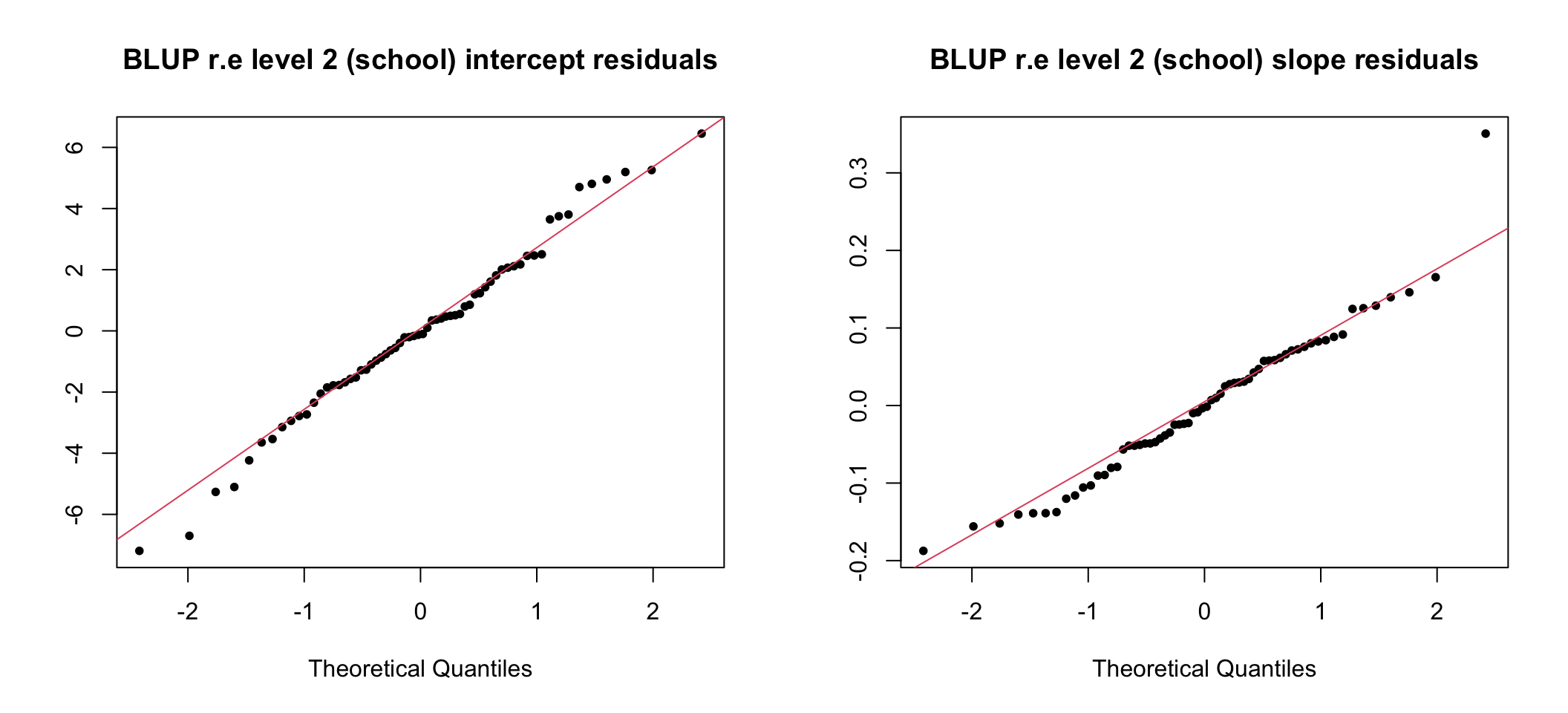
圖 75.4: Q-Q plots of school level intercept and slope residuals (unstandardized)
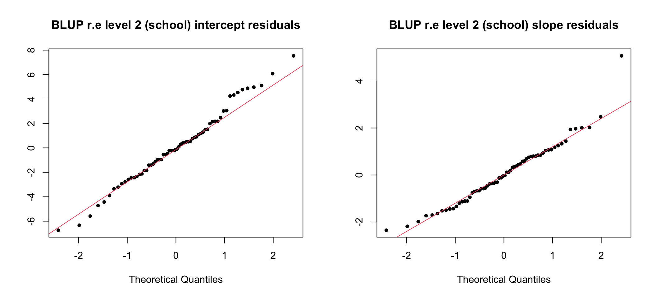
圖 75.5: Q-Q plots of school level intercept and slope residuals (standardized)
##  obs. mean   median  s.d.   min.   max.
##  4057 0      0.034   0.989  -3.832 3.455
圖 75.6: Histogram and Q-Q plots of elementary level (pupil) standardized residuals
75.7 Practical Hierarchical 04
- GCSE data: 數據來自65所中學的學生畢業成績 “the Graduate Certificate of Secondary Education (GCSE) score”,和這些學生在剛剛入學時接受閱讀能力水平測試 (LRT score) 的成績。其變量和各自含義爲:
school          school identifier
student         student identifier
gcse            GCSE score (multiplied by 10)
lrt             LRT score (multiplied by 10)
girl            Student female gender (1 = yes, 0 = no)
schgend         type of school (1: mixed gender; 2: boys only; 3: girls only)
### 將數據導入軟件裏,
gcse_selected <- read_dta("../backupfiles/gcse_selected.dta")

length(unique(gcse_selected$school)) ## number of school = 65
## [1] 65gcse_selected <- gcse_selected %>%
mutate(schgend = factor(schgend, labels = c("mixed geder", "boys only", "girls only")))
## create a subset data with only the first observation of each school
gcse <- gcse_selected[!duplicated(gcse_selected$school), ]
# 一共有 65 所學校,54% 是混合校,15% 是男校,31% 是女校
with(gcse, tab1(schgend, graph = FALSE))## schgend :
## Frequency Percent Cum. percent
## mixed geder 35 53.8 53.8
## boys only 10 15.4 69.2
## girls only 20 30.8 100.0
## Total 65 100.0 100.0# 計算每所學校兩種成績的平均分,計算一個包含每所學校的平均女生人數的變量
Mean_gcse_lrt <- ddply(gcse_selected,~school,summarise,mean_gcse=mean(gcse),mean_lrt=mean(lrt), mean_girl=mean(girl))
# 整體來說,GCSE 分數的分布比起入學前 LRT 分數的分布更加寬泛,標準差更大。
# 意味着入學時學生閱讀成績的差異,比起畢業時成績的差異要小。
# 或者反過來說,畢業時成績差異,比起入學時閱讀成績的差異要大。
epiDisplay::summ(Mean_gcse_lrt[,2:4])##
## No. of observations = 65
##
## Var. name obs. mean median s.d. min. max.
## 1 mean_gcse 65 -0.23 -0.34 4.39 -10.49 10.04
## 2 mean_lrt 65 -0.31 -0.41 3.44 -7.56 6.38
## 3 mean_girl 65 0.57 0.5 0.36 0 175.7.1 先忽略學校編號爲 48 的學校,擬合一個只有固定效應 (簡單線性回歸模型),結果變量是 GCSE,解釋變量是 LRT 和學校。
Fix <- lm(gcse ~ lrt + factor(school), data = gcse_selected[gcse_selected$school !=48, ])
anova(Fix)
## Analysis of Variance Table
##
## Response: gcse
## Df Sum Sq Mean Sq F value Pr(>F)
## lrt 1 141723.2 141723.2 2505.000 < 2.22e-16 ***
## factor(school) 63 37314.7 592.3 10.469 < 2.22e-16 ***
## Residuals 3992 225851.9 56.6
## ---
## Signif. codes: 0 '***' 0.001 '**' 0.01 '*' 0.05 '.' 0.1 ' ' 1LRT 的回歸系數 (直線斜率 = 0.56, se = 0.01),殘差的標準差 \(\hat\sigma_e =\) 7.52。
Call:
lm(formula = gcse ~ lrt + factor(school), data = gcse_selected[gcse_selected$school !=
    48, ])

Residuals:
   Min     1Q Median     3Q    Max
-28.32  -4.77   0.22   5.08  24.41

Coefficients:
                  Estimate Std. Error t value Pr(>|t|)
(Intercept)        4.08232    0.88060    4.64  3.7e-06 ***
lrt                0.55948    0.01253   44.63  < 2e-16 ***
factor(school)2    1.53785    1.34332    1.14  0.25235
                         ...
                         ...<OMITTED OUTPUT>
                         ...
                         ...
factor(school)65  -5.85245    1.21850   -4.80  1.6e-06 ***
---
Signif. codes:  0 ‘***’ 0.001 ‘**’ 0.01 ‘*’ 0.05 ‘.’ 0.1 ‘ ’ 1

Residual standard error: 7.52 on 3992 degrees of freedom
Multiple R-squared:  0.442, Adjusted R-squared:  0.433
F-statistic: 49.4 on 64 and 3992 DF,  p-value: <2e-16
75.7.2 僅有固定效應模型的學校變量變更爲學校類型 (男校女校或混合校),從這個新模型的結果來看,你是否認爲學校類型,和學校編號本身相比能夠解釋相同的學校層面的方差? lrt 的估計回歸參數發生了怎樣的變化?
## Analysis of Variance Table
##
## Response: gcse
##             Df   Sum Sq  Mean Sq   F value     Pr(>F)
## lrt          1 141723.2 141723.2 2222.6017 < 2.22e-16 ***
## schgend      2   4728.9   2364.4   37.0807 < 2.22e-16 ***
## Residuals 4053 258437.7     63.8
## ---
## Signif. codes: 0 '***' 0.001 '**' 0.01 '*' 0.05 '.' 0.1 ' ' 1##
## Call:
## lm(formula = gcse ~ lrt + schgend, data = gcse_selected[gcse_selected$school !=
## 48, ])
##
## Residuals:
## Min 1Q Median 3Q Max
## -26.17545 -5.12410 0.19171 5.35399 28.32233
##
## Coefficients:
## Estimate Std. Error t value Pr(>|t|)
## (Intercept) -0.960872 0.171460 -5.6041 2.233e-08 ***
## lrt 0.594272 0.012622 47.0836 < 2.2e-16 ***
## schgendboys only 1.177713 0.392041 3.0041 0.00268 **
## schgendgirls only 2.362920 0.275274 8.5839 < 2.2e-16 ***
## ---
## Signif. codes: 0 '***' 0.001 '**' 0.01 '*' 0.05 '.' 0.1 ' ' 1
##
## Residual standard error: 7.9853 on 4053 degrees of freedom
## Multiple R-squared: 0.36171, Adjusted R-squared: 0.36124
## F-statistic: 765.59 on 3 and 4053 DF, p-value: < 2.22e-16新的模型 Fix1 參數明顯減少很多,殘差標準差估計 \(\hat\sigma_u =\) 7.99。LRT 的回歸系數估計僅發生了不太明顯的變化 0.59 (0.01)
75.7.3 使用限制性極大似然法擬合一個隨機截距模型。記錄此時的限制性對數似然的大小 (log-likelihood)。用 lmerTest::rand 命令對隨機效應部分的方差是否爲零做檢驗,指明該檢驗的零假設是什麼,並解釋其結果的含義。
library(lmerTest)
Fixed_reml <- lmer(gcse ~ lrt +  (1 | school), data = gcse_selected[gcse_selected$school !=48, ], REML = TRUE)
summary(Fixed_reml)
## Linear mixed model fit by REML. t-tests use Satterthwaite's method ['lmerModLmerTest']
## Formula: gcse ~ lrt + (1 | school)
## Data: gcse_selected[gcse_selected$school != 48, ]
##
## REML criterion at convergence: 28044.1
##
## Scaled residuals:
## Min 1Q Median 3Q Max
## -3.71619 -0.63094 0.02920 0.68478 3.26661
##
## Random effects:
## Groups Name Variance Std.Dev.
## school (Intercept) 9.4273 3.0704
## Residual 56.6047 7.5236
## Number of obs: 4057, groups: school, 64
##
## Fixed effects:
## Estimate Std. Error df t value Pr(>|t|)
## (Intercept) 0.031006 0.405263 59.922917 0.0765 0.9393
## lrt 0.563268 0.012471 4048.045047 45.1676 <2e-16 ***
## ---
## Signif. codes: 0 '***' 0.001 '**' 0.01 '*' 0.05 '.' 0.1 ' ' 1
##
## Correlation of Fixed Effects:
## (Intr)
## lrt 0.007## ANOVA-like table for random-effects: Single term deletions
##
## Model:
## gcse ~ lrt + (1 | school)
## npar logLik AIC LRT Df Pr(>Chisq)
## <none> 4 -14022.0 28052.0
## (1 | school) 3 -14224.8 28455.7 405.601 1 < 2.22e-16 ***
## ---
## Signif. codes: 0 '***' 0.001 '**' 0.01 '*' 0.05 '.' 0.1 ' ' 1隨機截距模型的輸出結果可以看出,這裏的混合模型估計的 LRT 的回歸系數跟僅有固定效應的簡單線性回歸模型估計的值完全一樣 (0.56, se=0.01)。隨機效應部分 \(\hat\sigma_e = 7.524, \hat\sigma_u = 3.07\),此時的限制性似然 (restricted log-likelihood) 是 -14022。最晚部分的隨機效應檢驗的零假設是 \(\sigma_u = 0\),且值得注意的是,由於方差本身不可能小於零,故本次檢驗只用到自由度爲 1 的卡方分布的右半側(單側)。也就是說,其替代假設有且只有 \(\sigma_u > 0\) 的單側假設。這裏的檢驗結果提示高度有意義 (highly significant)。
75.7.4 在前一題的隨機截距模型中加入 schgend 變量,作爲解釋隨機截距的一個自變量,觀察輸出結果,解釋其是否有意義。記錄這個模型的限制性似然。
Fixed_reml1 <- lmer(gcse ~ lrt + schgend +  (1 | school), data = gcse_selected[gcse_selected$school !=48, ], REML = TRUE)
#Fixed_reml1 <- lme(fixed = gcse ~ lrt + schgend , random =  ~ 1 | school, data = gcse_selected[gcse_selected$school !=48, ], method = "REML")

summary(Fixed_reml1)
## Linear mixed model fit by REML. t-tests use Satterthwaite's method ['lmerModLmerTest']
## Formula: gcse ~ lrt + schgend + (1 | school)
## Data: gcse_selected[gcse_selected$school != 48, ]
##
## REML criterion at convergence: 28032.6
##
## Scaled residuals:
## Min 1Q Median 3Q Max
## -3.71222 -0.63023 0.02647 0.68064 3.24445
##
## Random effects:
## Groups Name Variance Std.Dev.
## school (Intercept) 8.4961 2.9148
## Residual 56.6045 7.5236
## Number of obs: 4057, groups: school, 64
##
## Fixed effects:
## Estimate Std. Error df t value Pr(>|t|)
## (Intercept) -0.872660 0.524979 58.504248 -1.6623 0.101807
## lrt 0.563512 0.012465 4049.316274 45.2087 < 2.2e-16 ***
## schgendboys only 0.968683 1.118170 59.752787 0.8663 0.389785
## schgendgirls only 2.497825 0.876614 56.676553 2.8494 0.006096 **
## ---
## Signif. codes: 0 '***' 0.001 '**' 0.01 '*' 0.05 '.' 0.1 ' ' 1
##
## Correlation of Fixed Effects:
## (Intr) lrt schgndbo
## lrt 0.006
## schgndbyson -0.469 0.006
## schgndgrlso -0.599 -0.004 0.281## 檢驗新增的學校種類 schgend 是否對應該加入模型。
mod2<- update(Fixed_reml1, . ~ . - schgend)
anova(Fixed_reml1, mod2)## Data: gcse_selected[gcse_selected$school != 48, ]
## Models:
## mod2: gcse ~ lrt + (1 | school)
## Fixed_reml1: gcse ~ lrt + schgend + (1 | school)
## npar AIC BIC logLik deviance Chisq Df Pr(>Chisq)
## mod2 4 28045.1 28070.4 -14018.6 28037.1
## Fixed_reml1 6 28041.1 28079.0 -14014.6 28029.1 8.01852 2 0.018147 *
## ---
## Signif. codes: 0 '***' 0.001 '**' 0.01 '*' 0.05 '.' 0.1 ' ' 1## 'log Lik.' -14016.32 (df=6)增加了學校類型在固定效應部分時,隨機效應的標準差從錢一個模型的 3.07 降低到這裏的 2.92。這個變量本身,從最後的模型比較也能看出,對模型的貢獻是有意義的 (p=0.018)。當然從隨機截距模型的輸出結果可以看出,學校類型的這一變量中,可能只有”女校”這一細分部分提供了足夠的效應。這裏的隨機截距模型的REML似然是 (restricted log-likelihood = -14016)
75.7.5 擬合隨機截距隨機斜率模型,固定效應部分的 lrt 也加入進隨機效應部分。
Fixed_reml2 <- lmer(gcse ~ lrt + schgend + (lrt | school), data = gcse_selected[gcse_selected$school !=48, ], REML = TRUE)## Warning in checkConv(attr(opt, "derivs"), opt$par, ctrl = control$checkConv, : Model failed to
## converge with max|grad| = 0.0350846 (tol = 0.002, component 1)## Linear mixed model fit by REML. t-tests use Satterthwaite's method ['lmerModLmerTest']
## Formula: gcse ~ lrt + schgend + (lrt | school)
## Data: gcse_selected[gcse_selected$school != 48, ]
##
## REML criterion at convergence: 27988.8
##
## Scaled residuals:
## Min 1Q Median 3Q Max
## -3.83030 -0.63006 0.03247 0.68532 3.41673
##
## Random effects:
## Groups Name Variance Std.Dev. Corr
## school (Intercept) 8.225497 2.86801
## lrt 0.014907 0.12209 0.582
## Residual 55.399136 7.44306
## Number of obs: 4057, groups: school, 64
##
## Fixed effects:
## Estimate Std. Error df t value Pr(>|t|)
## (Intercept) -1.09738 0.49633 63.43058 -2.2110 0.030648 *
## lrt 0.55823 0.02006 56.33412 27.8279 < 2.2e-16 ***
## schgendboys only 1.04115 0.99660 57.45922 1.0447 0.300536
## schgendgirls only 2.71117 0.78166 54.10008 3.4685 0.001035 **
## ---
## Signif. codes: 0 '***' 0.001 '**' 0.01 '*' 0.05 '.' 0.1 ' ' 1
##
## Correlation of Fixed Effects:
## (Intr) lrt schgndbo
## lrt 0.320
## schgndbyson -0.443 0.011
## schgndgrlso -0.566 0.011 0.284
## optimizer (nloptwrap) convergence code: 0 (OK)
## Model failed to converge with max|grad| = 0.0350846 (tol = 0.002, component 1)## 'log Lik.' -13994.393 (df=8)當截距 (不同學校之間, gcse 的起點),斜率 (不同學校之間 lrt 和 gcse 之間的關系的斜率) 均可以有隨機性以後,lrt 的斜率雖然仍然保持不變 \(=0.56\),但是它的隨機效應標準差變成了 \(=0.12\),隨機截距的標準差也保持不變 \(=2.88\),這二者之間的相關系數是 \(=0.58\)。第一階層隨機殘差標準也有了微妙的變化 \(7.52 \rightarrow 7.44\),此模型的限制性對數似然 (restricted log-likelihood) 是 -13994.393 (df=8)。
75.7.6 通過上面幾個模型計算獲得的似然,嘗試檢驗隨機斜率標準差,以及該標準差和隨機截距標準差的協相關是否有意義。
## ANOVA-like table for random-effects: Single term deletions
##
## Model:
## gcse ~ lrt + schgend + (lrt | school)
##                       npar   logLik     AIC     LRT Df Pr(>Chisq)
## <none>                   8 -13994.4 28004.8
## lrt in (lrt | school)    6 -14016.3 28044.6 43.8541  2 3.0006e-10 ***
## ---
## Signif. codes:  0 '***' 0.001 '**' 0.01 '*' 0.05 '.' 0.1 ' ' 1
# 手算的方法是這樣的
likelihood <- as.numeric(-2*(logLik(Fixed_reml1) - logLik(Fixed_reml2)))
0.5*(1-pchisq(as.numeric(likelihood), df = 1)) + 0.5*(1-pchisq(as.numeric(likelihood), df = 2))## [1] 1.6771939e-10似然比檢驗的統計量是 43.8,不用檢驗也知道肯定是有意義的。手算也是可以達到相同的效果。值得注意的是,R計算給出的基於自由度爲 2 的卡方分布,其實是偏保守的。注意看手算部分,其實用到了自由度爲 1 自由度爲 2 兩個卡方分布換算獲得的 p 值。
75.7.7 模型中的 schgend 改成 mean_girl 會給出怎樣的結果呢?
## 把女生平均值放回整體數據中去
Mean_girl <- NULL
for (i in 1:65) {
  Mean_girl <- c(Mean_girl, rep(Mean_gcse_lrt$mean_girl[i], with(gcse_selected, table(school))[i]))
  }
gcse_selected$mean_girl <- Mean_girl
  rm(Mean_girl)


Fixed_reml3 <- lmer(gcse ~ lrt + mean_girl +  (lrt | school), data = gcse_selected[gcse_selected$school !=48, ], REML = TRUE)
## Warning in checkConv(attr(opt, "derivs"), opt$par, ctrl = control$checkConv, : Model failed to
## converge with max|grad| = 0.0133558 (tol = 0.002, component 1)## Linear mixed model fit by REML. t-tests use Satterthwaite's method ['lmerModLmerTest']
## Formula: gcse ~ lrt + mean_girl + (lrt | school)
## Data: gcse_selected[gcse_selected$school != 48, ]
##
## REML criterion at convergence: 27997.1
##
## Scaled residuals:
## Min 1Q Median 3Q Max
## -3.81956 -0.63168 0.02994 0.68439 3.43510
##
## Random effects:
## Groups Name Variance Std.Dev. Corr
## school (Intercept) 8.910673 2.98507
## lrt 0.014913 0.12212 0.524
## Residual 55.388586 7.44235
## Number of obs: 4057, groups: school, 64
##
## Fixed effects:
## Estimate Std. Error df t value Pr(>|t|)
## (Intercept) -1.280011 0.705469 63.122736 -1.8144 0.07437 .
## lrt 0.556711 0.020084 56.134042 27.7190 < 2e-16 ***
## mean_girl 2.066161 1.031544 56.694088 2.0030 0.04997 *
## ---
## Signif. codes: 0 '***' 0.001 '**' 0.01 '*' 0.05 '.' 0.1 ' ' 1
##
## Correlation of Fixed Effects:
## (Intr) lrt
## lrt 0.220
## mean_girl -0.828 -0.004
## optimizer (nloptwrap) convergence code: 0 (OK)
## Model failed to converge with max|grad| = 0.0133558 (tol = 0.002, component 1)由於 mean_girl 其實是和 schgend 非常相似的表示學校層面的男女生性別比例的變量,所以這個模型的結果其實和前一個給出的隨機效應標準差的估計都很接近。
75.7.8 現在我們把注意力改爲關心學校編號爲 48 的學校的情況。用且禁用它一所學校的數據,擬合一個簡單線性回歸,結果變量是 gcse,解釋變量是 lrt。
## # A tibble: 2 × 7
##   school student  gcse   lrt  girl schgend    mean_girl
##    <dbl>   <dbl> <dbl> <dbl> <dbl> <fct>          <dbl>
## 1     48       1 -7.00 -3.73     1 girls only         1
## 2 48 2 -1.29 -4.55 1 girls only 1##
## Call:
## lm(formula = gcse ~ lrt, data = gcse_selected[gcse_selected$school ==
## 48, ])
##
## Residuals:
## ALL 2 residuals are 0: no residual degrees of freedom!
##
## Coefficients:
## Estimate Std. Error t value Pr(>|t|)
## (Intercept) -32.7221 NaN NaN NaN
## lrt -6.9018 NaN NaN NaN
##
## Residual standard error: NaN on 0 degrees of freedom
## Multiple R-squared: 1, Adjusted R-squared: NaN
## F-statistic: NaN on 1 and 0 DF, p-value: NA由於 48 號學校只有兩個數據點,所以強行進行簡單線性回歸的結果,就是擬合了一條通過這兩個點的直線,截距是-32.7,斜率是 -6.9,且沒有任何估計的誤差。
75.7.9 這次不排除 48 號學校,擬合所有學校的數據進入 Fixed_reml2 模型中去,結果有發生顯著的變化嗎?
## Warning in checkConv(attr(opt, "derivs"), opt$par, ctrl = control$checkConv, : Model failed to
## converge with max|grad| = 0.00818526 (tol = 0.002, component 1)## Linear mixed model fit by REML. t-tests use Satterthwaite's method ['lmerModLmerTest']
## Formula: gcse ~ lrt + schgend + (lrt | school)
## Data: gcse_selected
##
## REML criterion at convergence: 28001.4
##
## Scaled residuals:
## Min 1Q Median 3Q Max
## -3.83122 -0.63095 0.03275 0.68533 3.41855
##
## Random effects:
## Groups Name Variance Std.Dev. Corr
## school (Intercept) 8.248852 2.87208
## lrt 0.014968 0.12234 0.581
## Residual 55.376790 7.44156
## Number of obs: 4059, groups: school, 65
##
## Fixed effects:
## Estimate Std. Error df t value Pr(>|t|)
## (Intercept) -1.099128 0.496903 63.306279 -2.2120 0.030586 *
## lrt 0.558013 0.020081 56.230705 27.7876 < 2.2e-16 ***
## schgendboys only 1.041048 0.997647 57.338661 1.0435 0.301095
## schgendgirls only 2.672800 0.779708 54.625666 3.4280 0.001163 **
## ---
## Signif. codes: 0 '***' 0.001 '**' 0.01 '*' 0.05 '.' 0.1 ' ' 1
##
## Correlation of Fixed Effects:
## (Intr) lrt schgndbo
## lrt 0.321
## schgndbyson -0.443 0.011
## schgndgrlso -0.569 0.010 0.285
## optimizer (nloptwrap) convergence code: 0 (OK)
## Model failed to converge with max|grad| = 0.00818526 (tol = 0.002, component 1)可以看到,即使我們加入這個數據量極少的一個學校的數據,對結果也沒有太大的影響。
75.7.10 計算這個模型的第二階級(level 2, school level)的殘差。
School_res <- HLMdiag::hlm_resid(Fixed_reml2, level = "school", include.ls = FALSE)
epiDisplay::summ(School_res)
##
## No. of observations = 65
##
## Var. name obs. mean median s.d. min. max.
## 1 school
## 2 .ranef.intercept 65 0 0.11 2.65 -6.25 5.83
## 3 .ranef.lrt 65 0 0 0.1 -0.19 0.33## # A tibble: 1 × 3
## school .ranef.intercept .ranef.lrt
## <chr> <dbl> <dbl>
## 1 48 -0.739 -0.0147隨機截距的殘差估計範圍在 -6.25 和 5.83 之間,隨機斜率殘差估計範圍在 -0.19 和 0.33 之間。其中 48 號學校的擬合後截距和斜率分別是 -0.74 和 -0.02。48 號學校在這個模型中估計的截距和斜率,與我們單獨對它一所學校擬合模型時的結果大相徑庭。這是因爲在總體的混合效應模型中,該學校的數據被拉近與總體的平均水平。
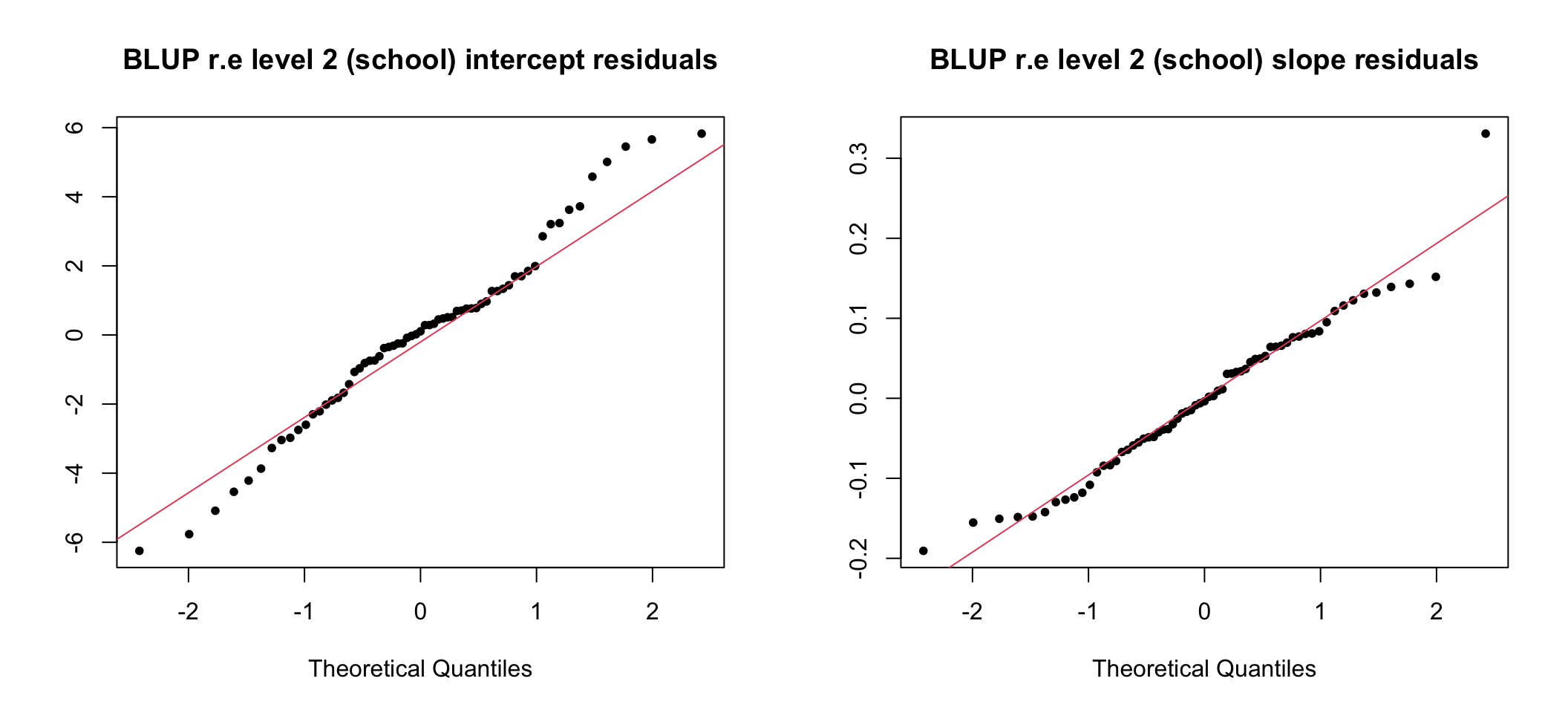
圖 75.7: Q-Q plots of school level intercept and slope (unstandardized) residuals
圖 75.7 顯示標準化前的隨機效應部分的殘差表現尚可接受。
75.7.11 計算這個模型的第一階級(level 1, student)殘差,分析其分布,查看第48所學校的殘差表現如何。
Fixed_reml2 <- lme(fixed = gcse ~ lrt + schgend, random = ~  lrt | school, data = gcse_selected, method="REML") # for extracting standardized level 2 error

gcse_selected$ehat <- residuals(Fixed_reml2, level = 1, type = "normalized")
with(gcse_selected, epiDisplay::summ(ehat, graph = FALSE))
## obs. mean median s.d. min. max.
## 4059 0 0.033 0.989 -3.831 3.419## 48 48
## -0.780061286 0.046827767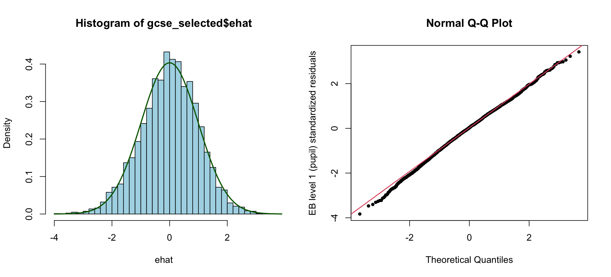
圖 75.8: Histogram and Q-Q plots of elementary level (pupil) standardized residuals