第 100 章 不同實驗/研究設計時適用的貝葉斯模型
本章節我們將要學習和探索如何給不同的實驗設計方法寫相對應的 BUGS 貝葉斯模型,用於比較不同組之間的差異。根據不同的試驗設計,模型也會跟着發生變化。例如病例對照研究的數據和模型結構,一定和隊列研究,或者是簡單的橫斷面研究的模型和數據結構差別甚遠。
爲不同的實驗設計寫下正確的貝葉斯模型的關鍵是,要深刻理解不同實驗設計時的樣本採集過程:實驗對象的哪些特徵,哪些變量是確定的,哪些被認爲是隨機變量。我們要爲那些被認爲是隨機變量的部分採集事後概率分佈樣本。
貫穿本章節,我們默認:
- \(Y\) 是要研究的疾病,\(X\) 是要研究的暴露因素;
- 給概率 (probabilities),和患病率 (prevalences)提供均一先驗概率分佈 (uniform priors)。給作用效果的評價指標例如危險度比 (risk ratios, RR),危險度差 (risk difference, RD),或者是比值比 (odds ratios, OR)提供中性的,圍繞着無效爲中心的先驗概率分佈 (“neutral” priors centred on no effect)。
100.1 隊列研究設計時的貝葉斯模型
假如我們徵集兩組觀察對象,一組爲2000名非吸菸者,另一組爲1000名吸菸者。他們年齡均爲30歲,之後我們隨訪這兩組研究對象20年,觀察到非吸菸者癌症發病人數爲100人,吸菸者癌症發病人數爲150人。這個實驗設計的目的是比較兩組觀察對象的20年癌症發病危險度。在這個實驗設計條件下,癌症發病是隨機變量,但是暴露組(吸菸)和非暴露組(非吸菸)的人數,是一開始已經定下來不會改變的數值。
需要強調的是,BUGS語言十分靈活,同一個模型,不同的人寫可能會給出完全不同,結果卻十分相近的代碼。給模型中的未知參數指定先驗概率分布時的方法也不盡相同。本隊列研究的實例中,比較癌症發病危險度 (risk) 的模型之一,可以寫作:
model{
    Y0 ~ dbin(r0, X0) # Data model for unexposed
    Y1 ~ dbin(r1, X1) # Data model for exposed

    # Priors for risks of exposed and unexposed
    r0 ~ dbeta(a.unexp, b.unexp)
    r1 ~ dbeta(a.exp, b.exp)

    # Computation of comparison statistics
    rd <-  r1 - r0   # for Risk Difference
    rr <- r1 / r0    # for Risk Ratio
}
數據文件可以寫作:
在上面的BUGS模型代碼中,我們需要給暴露組和非暴露組的發病危險度 (risks) 指定先驗概率分布。但是更常見的是直接給出危險度差,或者危險度比本身的先驗概率分布。這時候你可以把上面的 BUGS 模型加以修改:
model{
    Y0 ~ dbin(r0, X0) # Data model for unexposed
    Y1 ~ dbin(r1, X1) # Data model for exposed

    # define r1 as the unexposed risk plus an effect "rd"
    r1 <- r0 + rd

    # Priors for risks of exposed and unexposed
    r0 ~ dbeta(a.unexp, b.unexp)
    rd ~ dunif(min.rd, max.rd)

    # Computation of comparison statistics
    rr <- r1 / r0    # for Risk Ratio
}
對於這個模型代碼來說,你需要給出的數據文件中,對於 r1 的部分可以省去,但是需要給出 rd 的先驗概率分布中均一分布的兩個超參數 (hyper parameters):
如果你又改變主意,對相對危險度比 (risk ratio, RR) 的模型更加感興趣,建議你使用 logit 來把百分比放入模型中,因爲 \(\log \text{OR}\) 通常更加符合正態分布,便於給出先驗概率分布。這時候模型又可以變形成爲:
model{
    Y0 ~ dbin(r0, X0)   # Data model for unexposed
    logit(r0) <- lr0    # define the logit of r0
    Y1 ~ dbin(r1, X1)   # Data model for exposed
    logit(r1) <- lr1    # define the logit of r1

    # define lr1 as the unexposed logit(risk) plus log(OR):
    lr1 <- lr0 + lor

    # priors for the logit of risk of unexposed and of log(OR):
    lr0 ~ dnorm(mean.lr0, pr.lr0)
    lor ~ dnorm(mean.lor, pr.lor)

    # computations of comparison statistics:
    rd <- r1 - r0      # For risk difference
    rr <- r1 / r0      # For risk ratio
}
這個模型中要給 r0 一個均一分布的先驗概率,又希望給 or 指定一個95%可信區間在 (1/30, 30) 範圍內的先驗概率。那麼合適的數據文件可以寫作:
100.2 病例對照研究設計時的貝葉斯模型
假設試驗設計改成了病例對照研究,我們找到了1000名癌症患者,2000名無癌症的研究對象作爲對照。之後我們讓這兩羣研究對象回憶自己過去20年的吸煙史。假設數據收集到的是,在癌症患者組,有100名是吸煙者,在無癌症的對照組中吸煙人數有800人。在這個實驗設計的條件下,隨機會發生變化的就再也不是癌症的發病概率,或者危險度,而是吸煙於非吸煙的暴露,非暴露的變量 (smokers, non-smokers)。這時候我們來把模型中的變量用 logit 刻度(scale)來表示就是:
model{
    X0 ~ dbin(p0, Y0) # data model for CONTROLS
    logit(p0) <- lp0  # define the logit of p0
    X1 ~ dbin(p1, Y1) # data model for CASES
    logit(p1) <- lp1  # define the logit of p1

    # define lp1 as the unexposed logit(exposure) plus log(OR)
    lp1 <- lp0 + lor

    # Priors for logit of exposure and of log(OR)
    lp0 ~ dnorm(mean.lp0, pr.lp0)
    lor ~ dnorm(mean.lor, pr.lor)

    # Computation of comparison statistics
    or <- exp(lor)    # For Odds Ratio
}
這時候合適的數據文件,及先驗概率分布的超參數的指定可以寫作:
list(Y0 = 2000,
     Y1 = 1000,
     X0 = 800,
     X1 = 600,
     mean.lp0 = 0, pr.lp0 = 0.3,
     mean.lor = 0, pr.lor = 0.33)
從這裏的代碼也可以看出,此時我們能獲得的評價指標只能是比值比 OR,它直接從對數比值比\(\log \text{OR}\)獲得。在病例對照研究的實驗設計下,我們無法計算危險度差(risk difference),或者危險度比(risk ratio),因爲我們獲得的只有在病例組,和對照組中暴露和非暴露的百分比 (we only have probabilities of exposure in disease categories)。
100.3 橫斷面研究設計時的貝葉斯模型
思考橫斷面研究時,我們的數據是怎樣構成的?
此時我們採集400名實驗對象作爲橫斷面研究的樣本,然後在這個樣本中我們觀察他們的癌症患病與否,及吸煙習慣。假設數據是這樣的:
- 25名吸煙者患有癌症;
- 15名非吸煙者患有癌症;
- 150名吸煙者無癌症;
- 剩餘210名非吸煙者無癌症。
此時,這四個數據全部都是隨機變量。唯一一個固定不變的數字是總的樣本量 400 名研究對象。我們用 \(N_{ij}\) 來標記疾病狀態爲 \(i\),吸煙習慣爲 \(j\) 的實驗對象人數。其中 \(i, j = 0 \text{(absent) or } 1\text{(present)}\),那麼此時我們的數據就是 \(N=[N_{11}, N_{10}, N_{01}, N_{00}] = [25, 15, 150, 210]\)。
這四個數字是隨機,但不獨立的,因爲它們的總和400是已知的。這時可以想象這四個數字是按照一定的比例,從總體爲 1 的樣本中抽取,其參數分別是 \(\theta_{ij}, i, j = 0, 1\),且滿足 \(\sum_{ij}\theta_{ij} = 1\)。滿足這樣實驗設計的數學模型叫做多項式分布 (multinomial distribution):
\[ N \sim \text{Multinomial}([\theta_{11}, \theta_{10}, \theta_{01}, \theta_{00}], 400) \]
這樣的多項式分布中,我們感興趣的是其多個參數組成的一個互相有關系的向量 \(\mathbf{\theta}\)。由於這個向量中的參數之間並非相互獨立,所以我們無法分別一一給予先驗概率分布。(這很容易理解,因爲當某些參數很高時,其餘參數取值就必須是低的)這時候我們需要給整個向量 \(\mathbf{\theta}\) 提供一個綜合的先驗概率分布。
能給一個元素都是百分比的向量提供合適先驗概率的合理分布叫做狄利克雷 (Dirichlet) 分布。狄利克雷分布可以被認爲是 Beta 分布的多維擴展分布(multi-dimensional generalization of the beta distribution)。它是易於參數化(parameterize)的一個很靈活的分布,其組成元素就是一個由正數組成的向量 (a positive numbers):
\[ \mathbf{\theta} \sim \text{Dirichlet}(\alpha_1, \alpha_2, \dots. \alpha_k) \text{ where } \alpha_i >0, \text{ and we denote } \sum_{i = 1}^k \alpha_i = \alpha \]
一個滿足狄利克雷分布的向量,它有如下的特徵:
- 狄利克雷分布中的任意一個分類的(category)邊際先驗概率分布(marginal prior distribution)是一個Beta分布:\(\theta_i \sim \text{Beta}(\alpha_i, \alpha - \alpha_i)\);
- 狄利克雷分布中的任意一個分類的參數 \(\theta_i\) 的均值(期望)是:\(E(\theta_i) = \frac{\alpha_i}{\alpha}\);
- 狄利克雷分布中的任意一個分類的參數 \(\theta_i\) 的方差是:\(V(\theta_i) = \frac{E(\theta_i)(1-E(\theta_i))}{\alpha + 1}\)
另外有意思的一個特點是,當一個狄利克雷分布的所有元素 \(\alpha_i\) 同時乘以一個正數 \(w\) (positive number),產生的新的狄利克雷分布中的每個元素的參數均值(期望)與之前的狄利克雷分布均值相同,但是方差約等於之前狄利克雷分布元素的參數方差除以 \(w\)。利用這個性質,我們可以認爲 \(\alpha\) 相當於樣本量大小:
- 狄利克雷分布\(\text{Dirichlet}(1,2,1)\),其實是樣本量爲\(\alpha = 4\),均值是 \(\text{Means}[0.25, 0.5, 0.25]\)的分布;
- 狄利克雷分布\(\text{Dirichlet}(1,2,1)\),其實是樣本量爲\(\alpha = 40\),均值也是\(\text{Means}[0.25, 0.5, 0.25]\)的分布。
利用狄利克雷分布作爲橫斷面研究設計的先驗概率分布,我們把本節的實驗設計用BUGS語言總結出它的合適的模型:
model{
    N[1:4] ~ dmulti(p[], S)  # data model for sample
    p[1:4] ~ ddirch(alpha[]) # Dirichlet prior for vector of probabilities

    # Computation of comparison statistics:
    px0 <- p[2] + p[4]       # proportion of non-exposed
    px1 <- 1 - px0           # proportion of exposed
    r0 <- p[2] / px0         # risk in the non-exposed
    r1 <- p[1] / px1         # risk in the exposed
    rr <- r1 / r0            # risk ratio, RR
    rd <- r1 - r0            # risk difference, RD
    or <- (p[1]*p[4]) / (p[2]*p[3])   # odds ratio, OR
    p.crit <- step(or - 1)   # =1 if or >= 1, 0 otherwise

    # calculate the total sample size
    S <- sum(N[])
}
這個模型的數據文件則應該寫作:
模型的最後一行我們定義了總樣本量,且我們在橫斷面研究的實驗設計下,可以同時計算危險度差,危險度比,以及比值比等指標。另外我們還利用方便的step命令計算比值比大於1的概率。和其他任何一個貝葉斯模型一樣,我們需要給模型中的未知參數 p[1:4] 合理且分散的起始值 (initial values)。
這個模型的結果展示如下:
Iterations = 1001:26000
Thinning interval = 1
Number of chains = 2
Sample size per chain = 25000

1. Empirical mean and standard deviation for each variable,
   plus standard error of the mean:

             Mean       SD  Naive SE Time-series SE
deviance 18.81623 2.453005 1.097e-02      1.105e-02
or        2.43862 0.861082 3.851e-03      3.886e-03
p[1]      0.06436 0.012207 5.459e-05      5.459e-05
p[2]      0.03959 0.009694 4.335e-05      4.335e-05
p[3]      0.37378 0.024005 1.074e-04      1.078e-04
p[4]      0.52227 0.024829 1.110e-04      1.110e-04
p.crit    0.99372 0.078998 3.533e-04      3.630e-04
r0        0.07046 0.016980 7.594e-05      7.593e-05
r1        0.14689 0.026570 1.188e-04      1.188e-04
rd        0.07643 0.031454 1.407e-04      1.407e-04
rr        2.21362 0.703480 3.146e-03      3.172e-03

2. Quantiles for each variable:

             2.5%      25%      50%      75%    97.5%
deviance 16.04000 17.02000 18.19000 19.92000 25.11000
or        1.18700  1.83300  2.29700  2.88600  4.52103
p[1]      0.04272  0.05571  0.06368  0.07215  0.09039
p[2]      0.02285  0.03268  0.03880  0.04563  0.06050
p[3]      0.32720  0.35750  0.37360  0.38980  0.42150
p[4]      0.47350  0.50560  0.52240  0.53890  0.57060
p.crit    1.00000  1.00000  1.00000  1.00000  1.00000
r0        0.04094  0.05839  0.06914  0.08114  0.10730
r1        0.09882  0.12820  0.14570  0.16410  0.20270
rd        0.01569  0.05514  0.07586  0.09718  0.13970
rr        1.16700  1.71900  2.10500  2.58700  3.90200
可以看到,所有的監測指標的95%可信區間的下限都超過了零假設值 (null value)。且 OR 大於1的概率超過99%,由於我們使用的是無實際信息的先驗概率分布,所以這個分析結果是十分接近概率論模型的結果的。
假如我們現在有充分的理由相信,在本次研究對象中無癌症的對象中的吸煙者的百分比是被嚴重低估的,且我們有充足的理由認爲,這些人中有大約60%其實是吸煙者,但是對於癌症患者中吸煙者的百分比我們沒有太多的概念。那麼這樣的知識可以被翻譯到先驗概率分布的超參數裏面去:alpha = c(1,1,600,400)
這時候結果變成了下面這樣:
Iterations = 1001:26000
Thinning interval = 1
Number of chains = 2
Sample size per chain = 25000

1. Empirical mean and standard deviation for each variable,
   plus standard error of the mean:

             Mean       SD Naive SE Time-series SE
deviance 86.75869 10.43878 4.67e-02       4.67e-02
or        1.41233  0.48014 2.15e-03       2.15e-03
p[1]      0.01854  0.00361 1.61e-05       1.61e-05
p[2]      0.01141  0.00283 1.27e-05       1.28e-05
p[3]      0.53491  0.01330 5.95e-05       5.92e-05
p[4]      0.43514  0.01325 5.93e-05       5.96e-05
p.crit    0.81588  0.38759 1.73e-03       1.74e-03
r0        0.02554  0.00630 2.82e-05       2.86e-05
r1        0.03350  0.00646 2.89e-05       2.89e-05
rd        0.00796  0.00901 4.03e-05       4.03e-05
rr        1.39672  0.46134 2.06e-03       2.06e-03

2. Quantiles for each variable:

             2.5%      25%      50%     75%    97.5%
deviance 67.64000 79.50000 86.26000 93.5700 108.5000
or        0.70919  1.07600  1.33600  1.6600   2.5680
p[1]      0.01216  0.01598  0.01833  0.0208   0.0262
p[2]      0.00654  0.00940  0.01118  0.0132   0.0176
p[3]      0.50880  0.52600  0.53480  0.5439   0.5611
p[4]      0.40930  0.42620  0.43510  0.4440   0.4613
p.crit    0.00000  1.00000  1.00000  1.0000   1.0000
r0        0.01473  0.02106  0.02504  0.0294   0.0393
r1        0.02205  0.02894  0.03313  0.0376   0.0472
rd       -0.01009  0.00205  0.00804  0.0140   0.0255
rr 0.71649 1.07400 1.32400 1.6360 2.5040這時候我們通過先驗概率分布給模型中加入和較大的信息量,事實上,我們加入的先驗概率代表的”樣本量”:alpha = c(1,1,600,400),甚至比本次試驗本身的數據樣本量還要大。這時候各項指標 OR, RD, RR 的95%可信區間下限都包含了零假設值 (Null value)。甚至於此時OR大於1的概率已經降到了只有82%左右。
100.4 把不同實驗設計的數據用貝葉斯模型連接起來
通過使用不同的先驗概率分布,我們可以有效地利用實驗數據收集之前已經有的關於相似,或者相同實驗的重要結果(而不是僅僅做相互比較和討論)。比方說,我們計算獲得的某個模型某次實驗數據之後獲得的參數的事後概率分佈可以用作下一次類似研究時需要使用的先驗概率分佈信息。另外一種提高數據利用率的方法是,我們通過兩個試驗(可以是設計相同也可以是設計不同,但是討論相同研究問題的試驗)的共同參數把兩次甚至多次試驗的模型連接起來,如此既能提高事後概率分佈估計的精確度,也提高了數據的合理利用率。
100.4.1 Linking sub-models throug common parameters
在本章節的語境下,我們假設對一個相同的疾病結果\((Y)\),和相同的暴露因素\((X)\)之間的關係做了兩次不同的研究。數據分別收集自一個隊列研究,和一個病例對照研究。
對於隊列研究來說,我們用 \(X0c, X1c\) 分別標記非暴露組,及暴露組的總觀察人數;用 \(Y0c, Y1c\) 分別標記非暴露組和暴露組的新發病例人數。那麼和這個隊列研究數據分析相匹配的貝葉斯模型的 BUGS 代碼是:
model{
    # Data model for unexposed group
    Y0c ~ dbin(r0, X0c)
    logit(r0) <- lr0

    # Data model for exposed group
    Y1c ~ dbin(r1, X1c)
    logit(r1) <- lr1

    # lor is log(OR)
    lr1 <- lr0 + lor

    # Prior for logit of unexposed risk
    lr0 ~ dnorm(0, 0.3)
    # Prior for log(OR)
    lor ~ dnorm(0, 0.33)
}
該模型也可以用 DAG 有向無環圖 (100.1) 來表示:
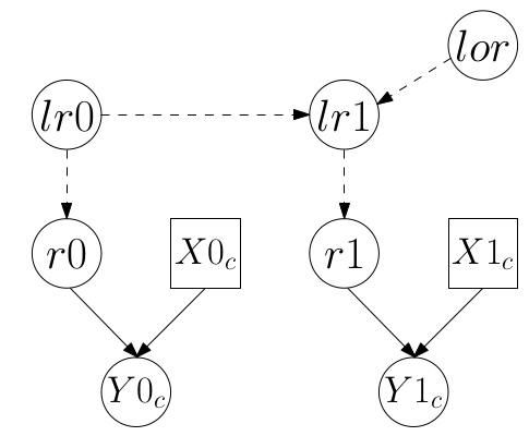
圖 100.1: DAG for model for data from the cohort study
至於病例對照設計的研究數據,用 \(Y0cc\) 來標記收集到的病例組人數,\(Y1cc\) 來標記收集到的對照組人數。用 \(X0cc, X1cc\) 分別標記對照組和病例組中有暴露的人數。那麼此時,該病例對照研究的實驗設計對應的BUGS語言描述的貝葉斯統計學模型可以寫作:
model{
    # Data model for controls
    X0cc ~ dbin(p0, Y0cc)
    logit(p0) <- lp0

    # Data model for cases
    X1cc ~ dbin(p1, Y1cc)
    logit(p1) <- lp1

    # lor is log(OR)
    lp1 <- lp0 + lor

    # Prior for logit of probability of exposure for controls
    lp0 ~ dnorm(0, 0.3)
    # Prior for log(OR)
    lor ~ dnorm(0, 0.33)
}
這個病例對照模型的 DAG 圖可以表示爲:
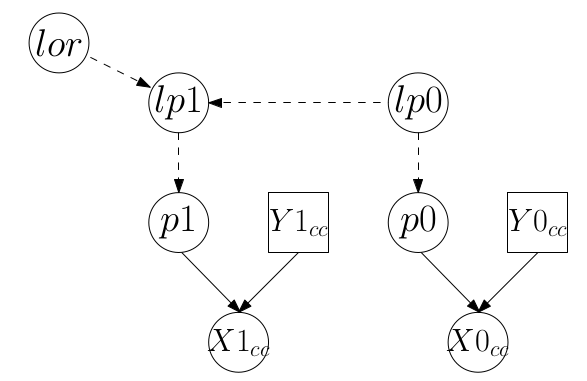
圖 100.2: DAG for model for data from the case-control study
從這兩個DAG圖我們也能一眼看出,這兩個模型裏面有一個共同的未知參數 lor。就是這個共同的參數可以讓我們把兩個模型連在一起,提高數據的利用效率。現在,我們把這兩個模型通過共同參數連起來的模型的DAG圖繪製出來:
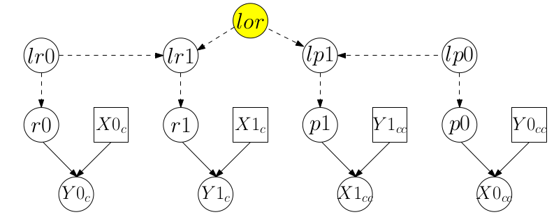
圖 100.3: DAG for JOINT model for data from the cohort study and the case-control study combined through log(OR)
此時,對應 DAG 圖 100.3 的合併模型的聯合模型,其BUGS語言描述的貝葉斯模型如下:
model{
# Cohort sub-model
   # Data model for unexposed group
    Y0c ~ dbin(r0, X0c)
    logit(r0) <- lr0

    # Data model for exposed group
    Y1c ~ dbin(r1, X1c)
    logit(r1) <- lr1

    # lor is log(OR)
    lr1 <- lr0 + lor

    # Prior for logit of unexposed risk
    lr0 ~ dnorm(0, 0.3)
# Case-control sub-model
   # Data model for controls
    X0cc ~ dbin(p0, Y0cc)
    logit(p0) <- lp0

    # Data model for cases
    X1cc ~ dbin(p1, Y1cc)
    logit(p1) <- lp1

    # lor is log(OR)
    lp1 <- lp0 + lor

    # Prior for logit of probability of exposure for controls
    lp0 ~ dnorm(0, 0.3)

# Prior for common log(OR)
    lor ~ dnorm(0, 0.33)
}
其實,通過類似的辦法,你可以把無數多個研究,無論它們是相似的或者不同的實驗設計,只要你能找到它們有共同的未知參數,就可以通過貝葉斯模型連接起來,成爲一個首尾相接,數據聯通的大模型。這真是一件在概率論模型下永遠也無法做到的神奇的事情!
100.5 Practical Bayesian Statistics 06
100.5.1 The GREAT Trial
在第一個章節,貝葉斯入門和回顧基礎知識的時候,我們介紹過GREAT臨牀試驗,這是一個雙盲對照試驗。比較阿尼普酶,一種血栓溶解藥物的兩種治療方案:
- 治療組:當患者被家庭醫生 (General Practitioners) 發現心肌梗塞時(myocardial infarctin, MI),在家中立刻給予阿尼普酶藥物,等到患者被救護車帶到醫院以後給患者服用安慰劑。
- 對照組:同樣情況下,家庭醫生在家中發現患者有心肌梗塞時先不給予藥物治療,而是先讓患者服用安慰劑,等救護車帶患者抵達醫院之後再讓患者服用真正的阿尼普酶藥物。
這項試驗的主要觀察結果 (primary outcome) 是30天死亡率。
該項試驗獲得的觀察數據如下:
- 治療組163人,13例死亡;
- 對照組148人,23例死亡。
利用這個簡單的臨牀試驗設定,我們來實際的體驗不同的先驗概率分佈對貝葉斯分析結果的影響。
我們用BUGS語言先描述這個模型的設定:
model {
    for (i in 1:2) {
        deaths[i] ~ dbin(p[i],n[i])
        logit(p[i]) <- alpha + beta*treat[i]
    }
    alpha ~ dunif(-100,100)
    beta ~ dunif(-100,100)
    OR <- exp(beta)
}
其中,
treat[i] 是一個指示变量 (indicator variable),i = 1 時表示對照組,i = 0 時表示治療組;
death[i] 是第 i 組對象的死亡病例數;
n[i]     是第 i 組對象的總人數;
p[i] 是第 i 組試驗組患者死亡的概率。- 解釋上面模型語句中
alpha, beta的含義是什麼。
alpha 是治療組的對數比值 (log odds for the treatment arm)
beta 是對照組和治療組相比較的死亡比值比 (log odds ratio of death in the control arm compared to the treatment arm),當 beta 大於1時,說明對照組死亡比值高,結果對治療組有利。
- 用兩組起始值文件來跑這個貝葉斯模型。
# Data file for the model
Dat <- list(
  n = c(163, 148),
  deaths = c(13, 23),
  treat = c(0, 1)
)

# initial values for the model
# the choice is arbitrary

inits <- list(
 list(alpha = 1, beta = -1),
 list(alpha = -1, beta = 1)
)

# fit the model in jags
jagsModel <- jags(data = Dat,
                  model.file = paste(bugpath,
                                  "/backupfiles/great-model1.txt",
                                  sep = ""),
                    parameters.to.save = c("OR", "alpha", "beta", "p"),
                     n.iter = 1000,
                     n.chains = 2,
                     inits = inits,
                     n.burnin = 0,
                     n.thin = 1,
                    progress.bar = "none")
## Compiling model graph
## Resolving undeclared variables
## Allocating nodes
## Graph information:
## Observed stochastic nodes: 2
## Unobserved stochastic nodes: 2
## Total graph size: 17
##
## Initializing model# Show the trace plot
Simulated <- coda::as.mcmc(jagsModel)
ggSample <- ggs(Simulated)
ggSample %>%
filter(Parameter %in% c("OR", "alpha", "beta", "p[1]", "p[2]")) %>%
ggs_traceplot()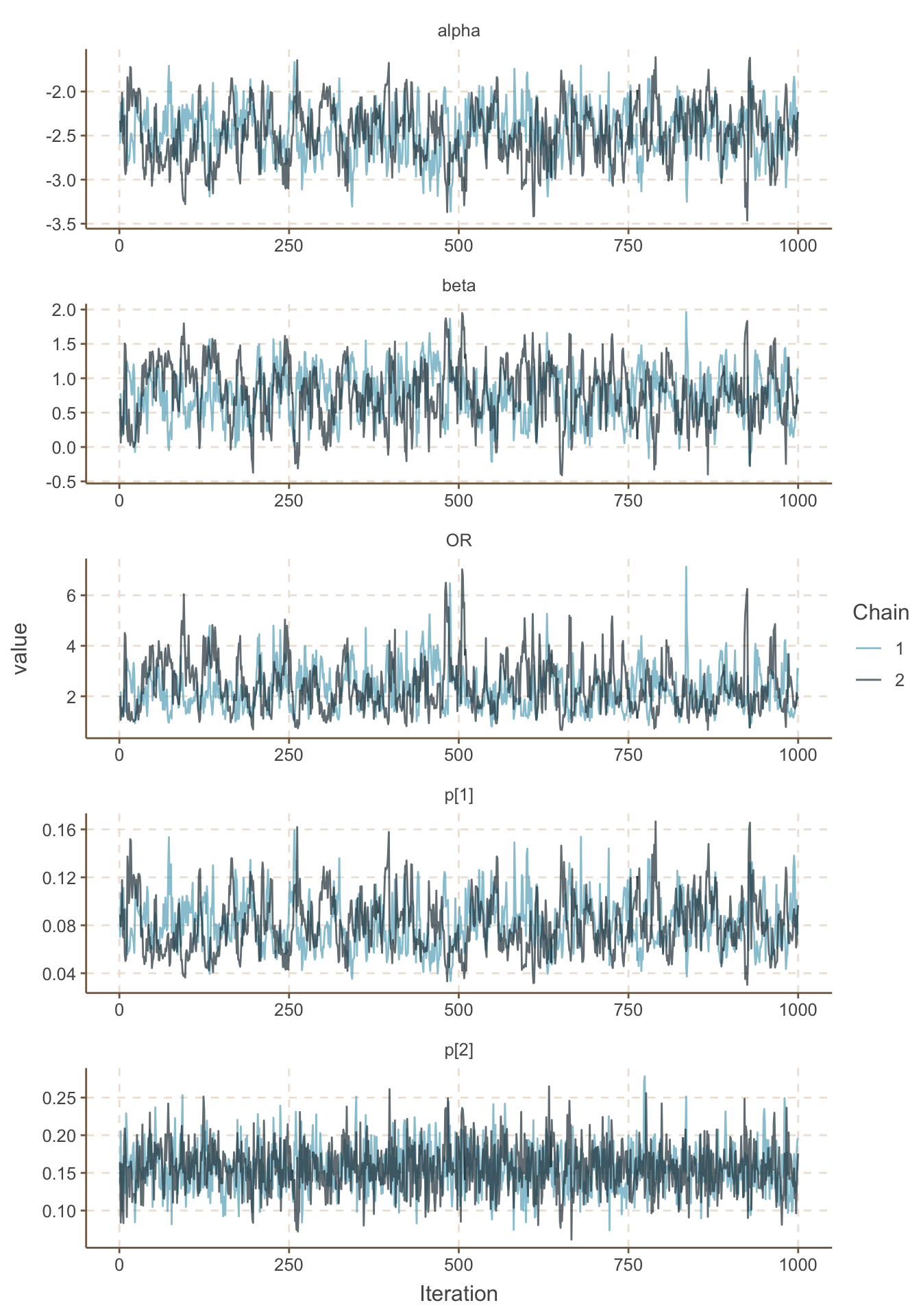
圖 100.4: History plots for iterations 1-1000 for the GREAT trial.
## Potential scale reduction factors:
##
##          Point est. Upper C.I.
## OR             1.05       1.13
## alpha          1.02       1.06
## beta           1.02       1.06
## deviance       1.02       1.07
## p[1]           1.01       1.04
## p[2]           1.00       1.01
##
## Multivariate psrf
##
## 1.02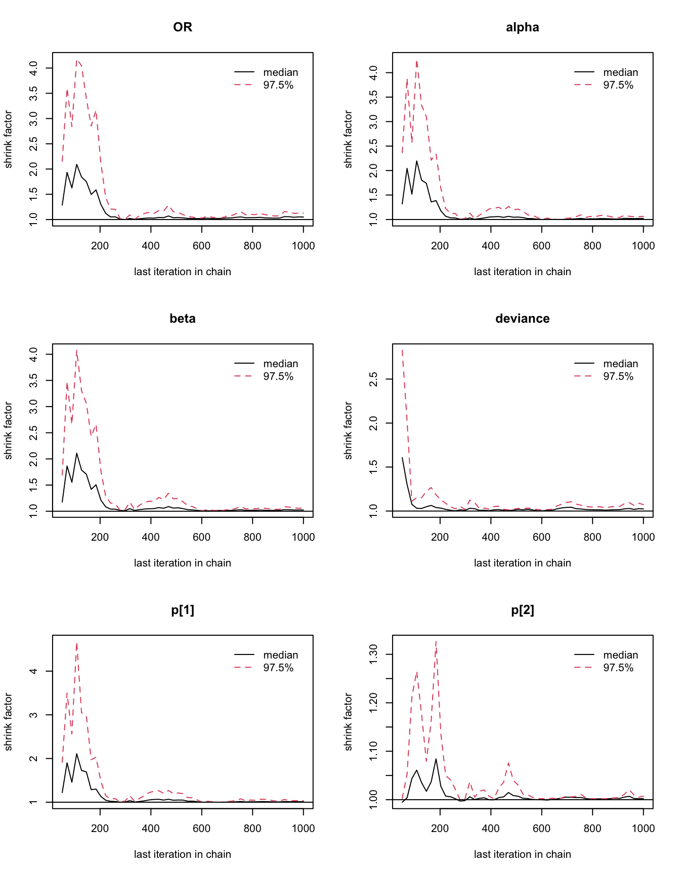
圖 100.5: Gelman-Rubin convergence statistic for the GREAT trial.
你會發現這個模型很快就能達到收斂,所以,我們選擇刨除前1000次採樣能夠滿足要求,我們另外再進行每條 MCMC 鏈各 25000 次樣本採集:
- 記錄這時候我們獲得的比值比 OR,迴歸係數,及兩組實驗組的事後死亡概率。
jagsModel <- jags(data = Dat,
                  model.file = paste(bugpath,
                                  "/backupfiles/great-model1.txt",
                                  sep = ""),
                    parameters.to.save = c("OR", "alpha", "beta", "p"),
                     n.iter = 26000,
                     n.chains = 2,
                     n.burnin = 1000,
                     n.thin = 1,
                     inits = inits,
                    progress.bar = "none")
## Compiling model graph
## Resolving undeclared variables
## Allocating nodes
## Graph information:
## Observed stochastic nodes: 2
## Unobserved stochastic nodes: 2
## Total graph size: 17
##
## Initializing model## Inference for Bugs model at "/Users/chaoimacmini/Downloads/LSHTMlearningnote/backupfiles/great-model1.txt", fit using jags,
## 2 chains, each with 26000 iterations (first 1000 discarded)
## n.sims = 50000 iterations saved
## mu.vect sd.vect 2.5% 25% 50% 75% 97.5% Rhat n.eff
## OR 2.315 0.915 1.058 1.674 2.144 2.760 4.606 1.001 35000
## alpha -2.480 0.295 -3.101 -2.669 -2.467 -2.277 -1.938 1.001 6000
## beta 0.769 0.373 0.057 0.515 0.763 1.015 1.527 1.001 35000
## p[1] 0.080 0.021 0.043 0.065 0.078 0.093 0.126 1.001 6000
## p[2] 0.155 0.030 0.102 0.135 0.154 0.174 0.218 1.001 16000
## deviance 11.164 2.024 9.197 9.725 10.540 11.938 16.601 1.001 50000
##
## For each parameter, n.eff is a crude measure of effective sample size,
## and Rhat is the potential scale reduction factor (at convergence, Rhat=1).
##
## DIC info (using the rule, pD = var(deviance)/2)
## pD = 2.0 and DIC = 13.2
## DIC is an estimate of expected predictive error (lower deviance is better).- 現在我們把先驗概率分佈修改成:
\[ \begin{aligned} \alpha & \sim \text{Logistic}(0,1) \\ \beta & \sim \text{Normal}(0, 0.33)\; 0.33 \text{ is the precision}\\ \end{aligned} \]
其中,邏輯分佈方程的BUGS語言是 dlogis;這個先驗概率給予 beta 的指定信息是基於想要給它一個沒有太多信息量的先驗概率分佈,其中對數比值比(log odds ratio)服從均值爲 0, 精確度(precision)爲 0.33 的正態分佈時,其對應的比值比 (odds ratio) 的95%則分佈在 1/30 至 30 之間。\((\text{sd} = \frac{\log30 - \log(1/30)}{2*1.96}) = 1.735 \rightarrow \tau^2 = (1/1.735)^2 \approx 0.33\)。
用相似的過程試着跑完這個貝葉斯模型:
jagsModel <- jags(data = Dat,
                  model.file = paste(bugpath,
                                  "/backupfiles/great-model1_alt.txt",
                                  sep = ""),
                    parameters.to.save = c("OR", "alpha", "beta", "p"),
                     n.iter = 1000,
                     n.chains = 2,
                     n.burnin = 0,
                     n.thin = 1,
                     inits = inits,
                    progress.bar = "none")
## Compiling model graph
## Resolving undeclared variables
## Allocating nodes
## Graph information:
## Observed stochastic nodes: 2
## Unobserved stochastic nodes: 2
## Total graph size: 18
##
## Initializing model# Show the trace plot
Simulated <- coda::as.mcmc(jagsModel)
ggSample <- ggs(Simulated)
ggSample %>%
filter(Parameter %in% c("OR", "alpha", "beta", "p[1]", "p[2]")) %>%
ggs_traceplot()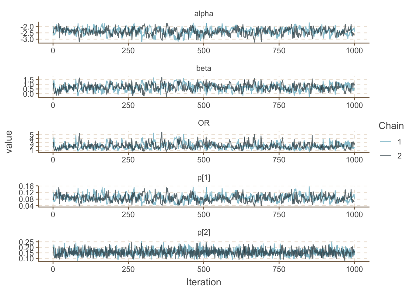
## Potential scale reduction factors:
##
##          Point est. Upper C.I.
## OR            1.020      1.078
## alpha         1.025      1.109
## beta          1.014      1.069
## deviance      1.000      1.000
## p[1]          1.021      1.099
## p[2]          0.999      0.999
##
## Multivariate psrf
##
## 1.02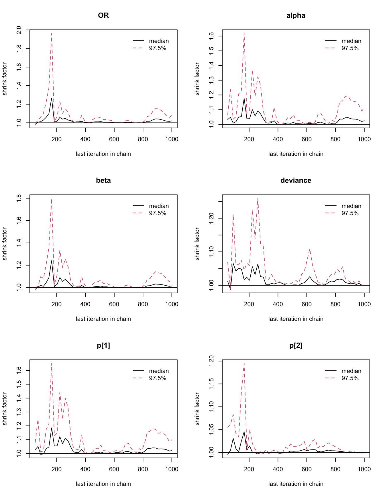
圖 100.6: Gelman-Rubin convergence statistic for the GREAT trial with alternative priors for alpha and beta.
jagsModel <- jags(data = Dat,
                  model.file = paste(bugpath,
                                  "/backupfiles/great-model1_alt.txt",
                                  sep = ""),
                    parameters.to.save = c("OR", "alpha", "beta", "p"),
                     n.iter = 26000,
                     n.chains = 2,
                     n.burnin = 1000,
                     n.thin = 1,
                     inits = inits,
                    progress.bar = "none")
## Compiling model graph
## Resolving undeclared variables
## Allocating nodes
## Graph information:
## Observed stochastic nodes: 2
## Unobserved stochastic nodes: 2
## Total graph size: 18
##
## Initializing model## Inference for Bugs model at "/Users/chaoimacmini/Downloads/LSHTMlearningnote/backupfiles/great-model1_alt.txt", fit using jags,
## 2 chains, each with 26000 iterations (first 1000 discarded)
## n.sims = 50000 iterations saved
## mu.vect sd.vect 2.5% 25% 50% 75% 97.5% Rhat n.eff
## OR 2.086 0.779 0.977 1.536 1.950 2.478 3.993 1.001 4700
## alpha -2.393 0.279 -2.979 -2.575 -2.381 -2.199 -1.879 1.001 5100
## beta 0.671 0.357 -0.023 0.429 0.668 0.907 1.385 1.001 4700
## p[1] 0.086 0.022 0.048 0.071 0.085 0.100 0.133 1.001 5200
## p[2] 0.154 0.029 0.101 0.133 0.153 0.173 0.215 1.001 30000
## deviance 11.129 1.976 9.192 9.718 10.526 11.893 16.403 1.001 38000
##
## For each parameter, n.eff is a crude measure of effective sample size,
## and Rhat is the potential scale reduction factor (at convergence, Rhat=1).
##
## DIC info (using the rule, pD = var(deviance)/2)
## pD = 2.0 and DIC = 13.1
## DIC is an estimate of expected predictive error (lower deviance is better).- 對改變了先驗概率前後的貝葉斯分析結果,你有什麼看法?
我們發現改變先驗概率前的模型得到的事後比值比的結果有更大的均值,及更不穩定的估計(較高的事後樣本標準差,及較寬的事後樣本95%可信區間)。
- 爲了分析改變先驗概率分佈前後到底哪種給予了模型更多的信息,我們可以把兩個模型改寫成不含數據,只有預測模型的語句,從而可以看到只有先驗概率分佈時的結果是怎樣的。這時候我們把數據加載這一步省略掉,然後對
alpha, beta, p進行軌跡檢測,繪製他們的預測分佈密度曲線。
library(runjags)
library(rjags)
library(R2jags)

# Step 1 check model
jagsModel <- jags.model(file = paste(bugpath, "/backupfiles/great-model1_forward.txt", sep = ""),
                        data = list(treat = c(0, 1)),
                        n.chains = 2)
## Compiling model graph
## Resolving undeclared variables
## Allocating nodes
## Graph information:
## Observed stochastic nodes: 0
## Unobserved stochastic nodes: 2
## Total graph size: 13
##
## Initializing model# Step 2 update 1000 iterations
update(jagsModel, n.iter = 25000, progress.bar="none")
# Step 3 set monitor variables
codaSamples <- coda.samples(
jagsModel,
variable.names = c("alpha", "beta", "p[1]", "p[2]"),
n.iter = 25000, progress.bar="none")
# Show density plot
mcmcplots::denplot(codaSamples)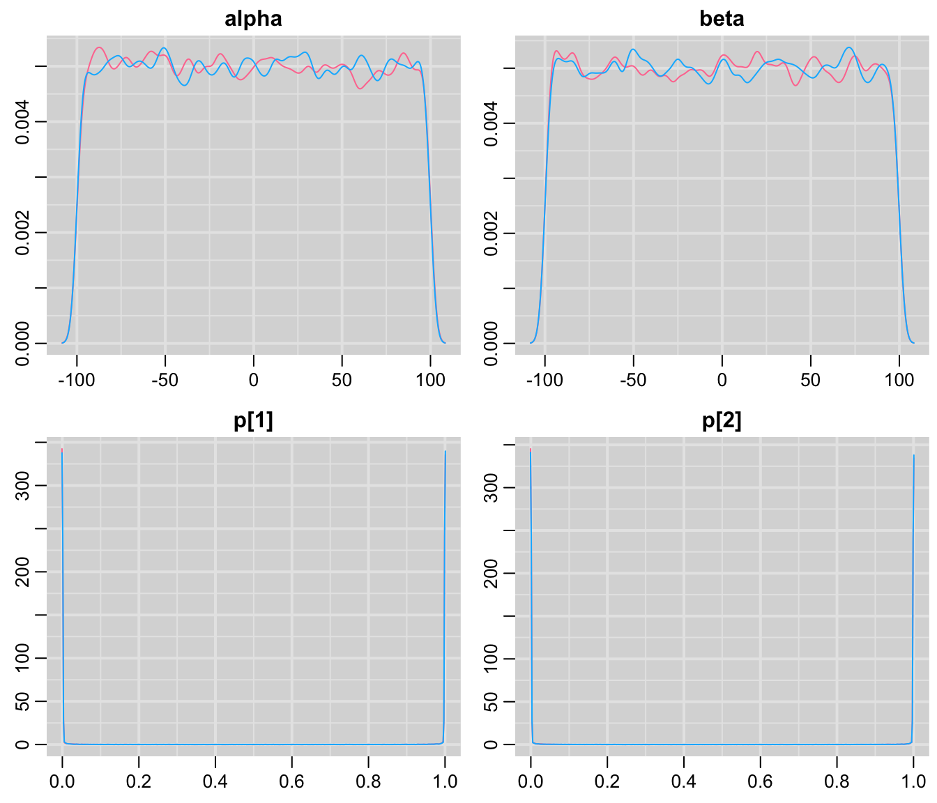
圖 100.7: Density plots for parameters prediction in GREAT trial first prior.
# ggSample <- ggs(codaSamples)
# ggSample %>%
#   filter(Parameter %in% c("alpha", "beta", "p[1]", "p[2]")) %>%
#   ggs_density()
對於這個模型來說,儘管我們給兩個邏輯迴歸的參數 alpha, beta 兩個”沒有信息”的均一分佈 (uniform distribution) 作爲先驗概率分佈,但是事實上,從 p[1], p[2] 的預測概率密度分佈圖來看,其實我們不經意竟然告訴模型另外的信息:就是我們認爲這兩組患者中死亡率要麼很高,接近1,要麼很低很低,接近於0。所以,我們自認爲給了模型無信息的先驗概率分佈,但是事實上卻給了模型大量的信息。
# Step 1 check model
jagsModel <- jags.model(file = paste(bugpath, "/backupfiles/great-model1_altforward.txt", sep = ""),
                        data = list(treat = c(0, 1)),
                        n.chains = 2)
## Compiling model graph
## Resolving undeclared variables
## Allocating nodes
## Graph information:
## Observed stochastic nodes: 0
## Unobserved stochastic nodes: 2
## Total graph size: 14
##
## Initializing model# Step 2 update 1000 iterations
update(jagsModel, n.iter = 25000, progress.bar="none")
# Step 3 set monitor variables
codaSamples <- coda.samples(
jagsModel,
variable.names = c("alpha", "beta", "p[1]", "p[2]"),
n.iter = 25000, progress.bar="none")
# Show density plot
mcmcplots::denplot(codaSamples)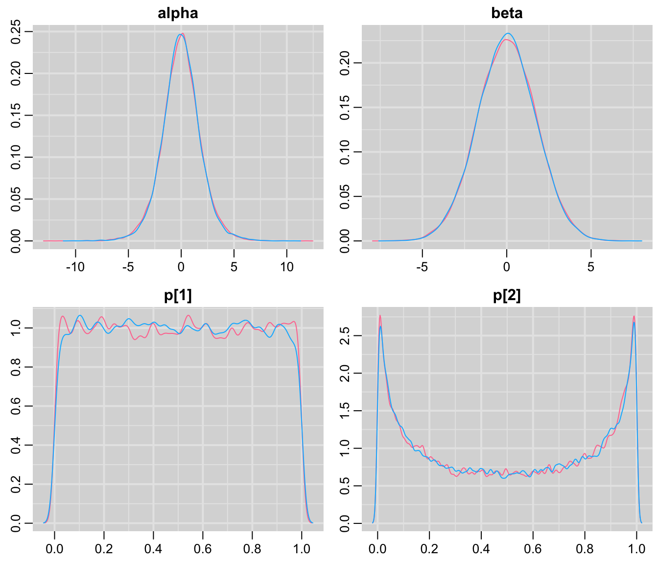
圖 100.8: Density plots for parameters prediction in GREAT trial second prior.
第二次修改過後的先驗概率明顯就安全得多了。因爲我們看到兩組的死亡概率基本可以認爲不再像前一個模型那樣含有太多不實際的信息。
- 作爲替代方案,我們可以把上述模型重新用對數比值比(Log odds ratio, LOR)作爲未知參數來重新建模:
\[ LOR = \log(\frac{p[1]/(1 - p[1])}{p[2]/(1 - p[2])}) = \text{logit}(p[1]) - \text{logit}(p[2]) \]
這時候我們需要給 p[2], LOR 賦予先驗概率分布:
model {
    for (i in 1:2) {
        deaths[i] ~ dbin(p[i],n[i])
    }
    logit(p[1]) <- logit(p[2]) + LOR
    p[2] ~ dbeta(1,1)
    LOR ~ dnorm(0,0.33)
    OR <- exp(LOR)
}- 再看一遍上面寫好的模型,確定你能夠理解其含義,請確認先驗概率分布的實際意義。
注意我們用beta 分布來描述 p[2] 的先驗概率分布。
jagsModel <- jags(data = list(n = c(148, 163), deaths = c(23, 13)),
                  model.file = paste(bugpath,
                                  "/backupfiles/great-model2.txt",
                                  sep = ""),
                    parameters.to.save = c("OR", "p"),
                     n.iter = 26000,
                     n.chains = 2,
                     n.burnin = 1000,
                     n.thin = 1,
                     inits = list(list(LOR = 0.5, p = c(NA, 0.2)),
                                  list(LOR = 5, p = c(NA, 0.8))),
                    progress.bar = "none")
## Compiling model graph
## Resolving undeclared variables
## Allocating nodes
## Graph information:
## Observed stochastic nodes: 2
## Unobserved stochastic nodes: 2
## Total graph size: 13
##
## Initializing model## Inference for Bugs model at "/Users/chaoimacmini/Downloads/LSHTMlearningnote/backupfiles/great-model2.txt", fit using jags,
## 2 chains, each with 26000 iterations (first 1000 discarded)
## n.sims = 50000 iterations saved
## mu.vect sd.vect 2.5% 25% 50% 75% 97.5% Rhat n.eff
## OR 2.085 0.777 0.988 1.541 1.949 2.476 3.975 1.001 7700
## p[1] 0.154 0.029 0.101 0.133 0.152 0.173 0.215 1.001 21000
## p[2] 0.086 0.021 0.049 0.071 0.084 0.099 0.132 1.001 12000
## deviance 11.119 1.978 9.193 9.716 10.511 11.864 16.425 1.001 5500
##
## For each parameter, n.eff is a crude measure of effective sample size,
## and Rhat is the potential scale reduction factor (at convergence, Rhat=1).
##
## DIC info (using the rule, pD = var(deviance)/2)
## pD = 2.0 and DIC = 13.1
## DIC is an estimate of expected predictive error (lower deviance is better).- 修改模型的代碼使之用於向前採集樣本用於預測:
model {
#   for (i in 1:2) {
#       deaths[i] ~ dbin(p[i],n[i])
#   }
    logit(p[1]) <- logit(p[2]) + LOR
    p[2] ~ dbeta(1,1)
    LOR ~ dnorm(0,0.33)
    OR <- exp(LOR)
}
# Step 1 check model
jagsModel <- jags.model(file = paste(bugpath, "/backupfiles/great-model2_forward.txt", sep = ""),
n.chains = 2)## Compiling model graph
## Resolving undeclared variables
## Allocating nodes
## Graph information:
## Observed stochastic nodes: 0
## Unobserved stochastic nodes: 2
## Total graph size: 9
##
## Initializing model# Step 2 update 1000 iterations
update(jagsModel, n.iter = 25000, progress.bar="none")
# Step 3 set monitor variables
codaSamples <- coda.samples(
jagsModel,
variable.names = c("p[1]", "p[2]"),
n.iter = 25000, progress.bar="none")
# Show density plot
mcmcplots::denplot(codaSamples)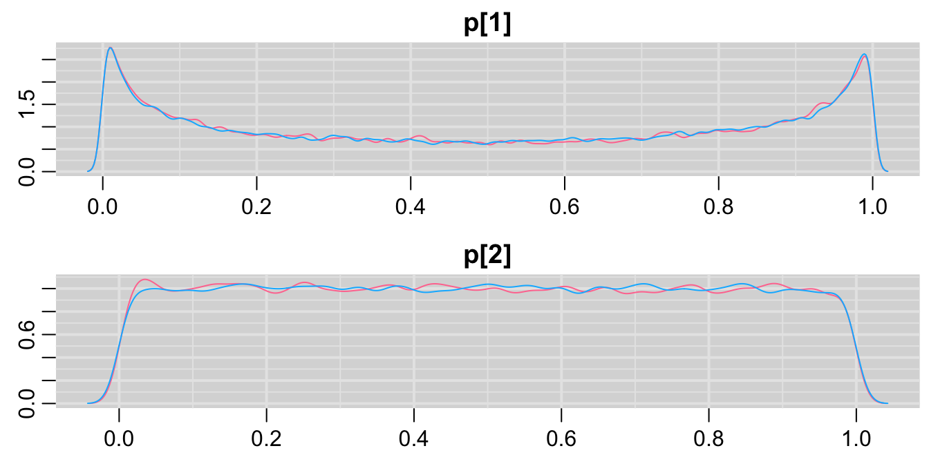
圖 100.9: Density plots for parameters prediction in GREAT trial second prior.
這時候先驗概率分布給出的兩組死亡率的密度分布和之前提出的第二個模型沒有什麼兩樣。
100.5.2 吸煙與癌症
在這道題中,你將練習自己使用和描述一個隊列研究設計,及一個病例對照研究設計的貝葉斯模型,同時學習如何把兩個試驗的數據和模型通過共同的未知參數連接起來。在整道題目中,癌症作爲發病結果 (disease of interest),吸煙作爲暴露因素 (exposure of interest)。
100.5.2.1 隊列研究設計
在一個隊列研究中,2000名非吸煙者,和1000名吸煙者被跟蹤隨訪20年。在非吸煙者中和非吸煙者中分別觀察到100例,及150例新發生的癌症患者。我們關心的是和非吸煙者相比,吸煙者患癌症的比值比是多少。這個實驗的貝葉斯模型可以寫作:
model{
    # Data model for non-smokers
    Y0c ~ dbin(r0, X0c)
    logit(r0) <- lr0

     # Data model for smokers
     Y1c ~ dbin(r1, X1c)
     logit(r1) <- lr1

    lr1 <- lr0 + lor   # lor is log(OR)
    OR <- exp(lor)  # comparison statistic

    # Priors
    lr0 ~ dnorm(0, 0.3)  # priors for logit of non-smokers
    lor ~ dnorm(0, 0.33)  # prior for log(OR)
}


# Y0c number of non-smokers developed cancer
# X0c number of nonpsmokers
# Y1c number of smokers developed cancer
# X1c number of smokers
數據文件可以寫作:
list(X0c = 2000,
     Y0c = 100,
     X1c = 1000,
     Y1c = 150)
未知參數 lor, lr0 的起始值可以選定爲:
list(lr0 = -1, lor = 0)
list(lr0 = -5, lor = 5)
對這個模型進行50000次事後樣本採集,獲取比值比 OR 的事後概率分布描述:
# Data file for the model
Dat <- list(
  X0c = 2000,
  Y0c = 100,
  X1c = 1000,
  Y1c = 150
)

# initial values for the model
# the choice is arbitrary

inits <- list(
 list(lr0 = -1, lor = 0),
 list(lr0 = -5, lor = 5)
)

# fit the model in jags
jagsModel <- jags(data = Dat,
                  model.file = paste(bugpath,
                                  "/backupfiles/cohort-model.txt",
                                  sep = ""),
                    parameters.to.save = c("OR", "lor"),
                     n.iter = 1000,
                     n.chains = 2,
                     inits = inits,
                     n.burnin = 0,
                     n.thin = 1,
                    progress.bar = "none")
## Compiling model graph
## Resolving undeclared variables
## Allocating nodes
## Graph information:
## Observed stochastic nodes: 2
## Unobserved stochastic nodes: 2
## Total graph size: 13
##
## Initializing model# Show the trace plot
Simulated <- coda::as.mcmc(jagsModel)
ggSample <- ggs(Simulated)
ggSample %>%
filter(Parameter %in% c("OR", "lor")) %>%
ggs_traceplot()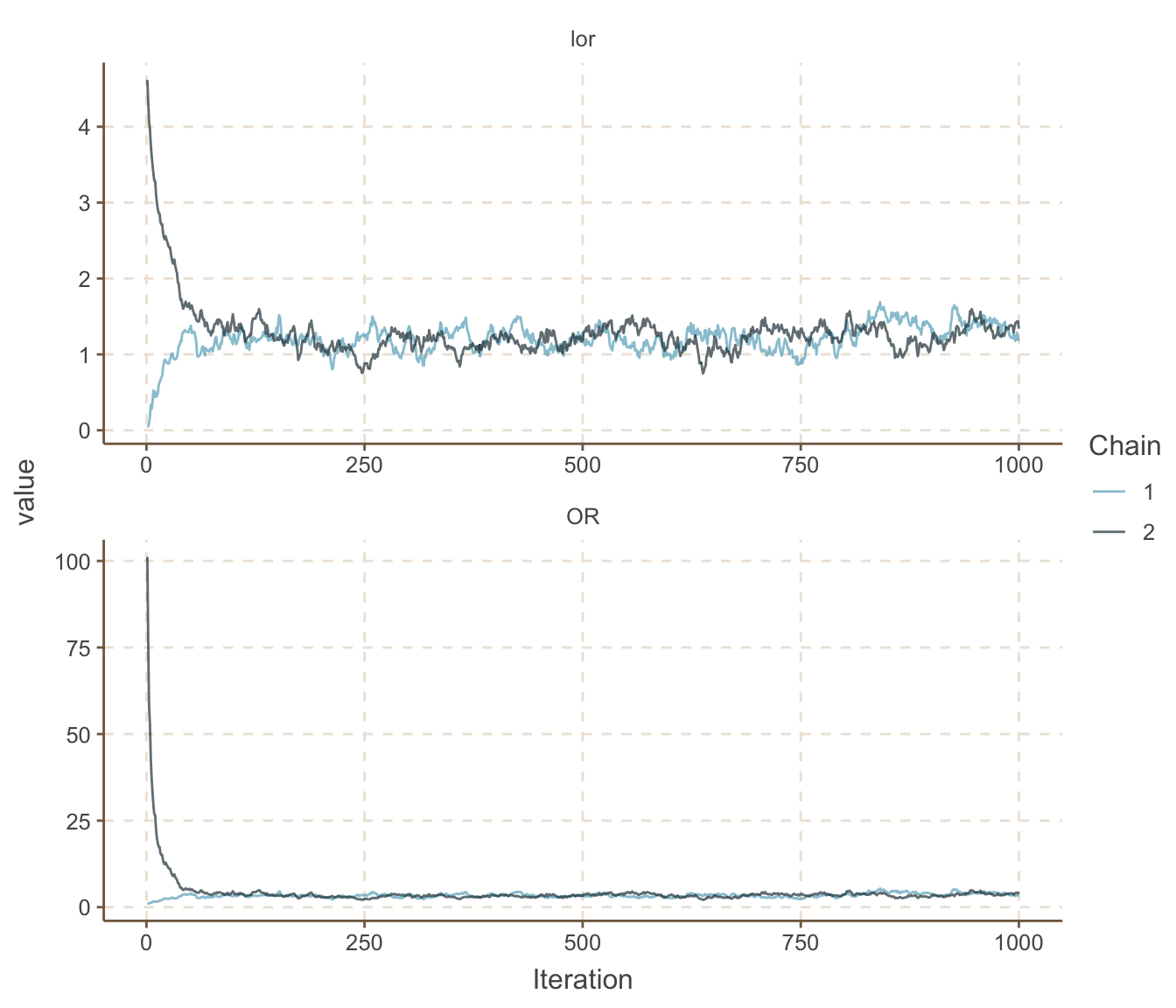
圖 100.10: Density plots for parameters prediction in smoking and cancer cohort study.
## Potential scale reduction factors:
##
##          Point est. Upper C.I.
## OR             1.02       1.02
## deviance       1.10       1.30
## lor            1.01       1.01
##
## Multivariate psrf
##
## 1.04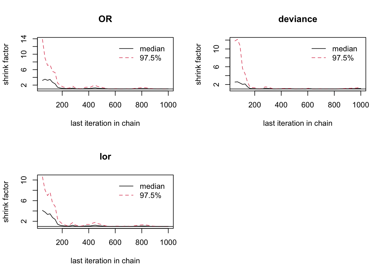
圖 100.11: Gelman-Rubin convergence statistic for smoking and cancer cohort study.
jagsModel <- jags(data = Dat,
                  model.file = paste(bugpath,
                                  "/backupfiles/cohort-model.txt",
                                  sep = ""),
                    parameters.to.save = c("OR", "lor"),
                     n.iter = 26000,
                     n.chains = 2,
                     inits = inits,
                     n.burnin = 1000,
                     n.thin = 1,
                    progress.bar = "none")
## Compiling model graph
## Resolving undeclared variables
## Allocating nodes
## Graph information:
## Observed stochastic nodes: 2
## Unobserved stochastic nodes: 2
## Total graph size: 13
##
## Initializing model## Inference for Bugs model at "/Users/chaoimacmini/Downloads/LSHTMlearningnote/backupfiles/cohort-model.txt", fit using jags,
## 2 chains, each with 26000 iterations (first 1000 discarded)
## n.sims = 50000 iterations saved
## mu.vect sd.vect 2.5% 25% 50% 75% 97.5% Rhat n.eff
## OR 3.354 0.870 2.554 3.023 3.310 3.625 4.306 1.008 9800
## lor 1.198 0.143 0.938 1.106 1.197 1.288 1.460 1.001 19000
## deviance 15.252 7.075 13.130 13.666 14.482 15.836 20.431 1.007 3900
##
## For each parameter, n.eff is a crude measure of effective sample size,
## and Rhat is the potential scale reduction factor (at convergence, Rhat=1).
##
## DIC info (using the rule, pD = var(deviance)/2)
## pD = 25.0 and DIC = 40.3
## DIC is an estimate of expected predictive error (lower deviance is better).100.5.2.2 病例對照研究設計下的模型
在病例對照研究設計下,研究者收集了1000名癌症患者(病例組),和2000名對照組志願者。研究者對這兩組研究對象分別調查了他們各自過去20年的吸煙史,發現:
- 病例組中600人過去20年中有過吸煙史;
- 對照組中800人過去20年中有過吸煙史。
同樣地,我們關心的是兩組之間吸煙習慣的比值比 (Odds ratio)。這個實驗設計的模型可以用BUGS語言寫作(保存爲case-control-model.txt):
model{
    # Data model for non-cancer controls
    X0cc ~ dbin(p0, Y0cc)
    logit(p0) <- lp0

    # Data model for cancer cases
     X1cc ~ dbin(p1, Y1cc)
    logit(p1) <- lp1

    lp1 <- lp0 + lor # lor is log(OR)
    OR <- exp(lor)  # comparison statistic

     # Priors
     lp0 ~ dnorm(0, 0.3)  # prior for logit of probability of exposure for controls
     lor ~ dnorm(0, 0.33) # prior for log(OR)
    }


    # X0cc indicates number of smokers among controls (without cancer)
    # Y0cc indicates number of controls
    # X1cc is the number of smokers among cancer cases
    # Y1cc is the number of cancer cases
其中,
X0cc表示對照組中有吸煙史的人數;Y0cc表示對照組的總人數;X1cc表示癌症患者組中有吸煙史的人數;Y1cc表示癌症患者組的總人數。
數據文件可以描述爲(保存爲dataforcasecontrol.txt):
list(X0cc = 800,
     Y0cc = 2000,
     X1cc = 600,
     Y1cc = 1000)
模型擬合過程和結果分別羅列如下:
# Data file for the model
Dat <- list(X0cc = 800,
            Y0cc = 2000,
            X1cc = 600,
            Y1cc = 1000)

# initial values for the model
# the choice is arbitrary

inits <- list(
 list(lp0 = -2, lor = 0),
 list(lp0 = 2, lor = 5)
)

# fit the model in jags
jagsModel <- jags(data = Dat,
                  model.file = paste(bugpath,
                                  "/backupfiles/case-control-model.txt",
                                  sep = ""),
                    parameters.to.save = c("OR", "lor"),
                     n.iter = 1000,
                     n.chains = 2,
                     inits = inits,
                     n.burnin = 0,
                     n.thin = 1,
                    progress.bar = "none")
## Compiling model graph
## Resolving undeclared variables
## Allocating nodes
## Graph information:
## Observed stochastic nodes: 2
## Unobserved stochastic nodes: 2
## Total graph size: 13
##
## Initializing model# Show the trace plot
Simulated <- coda::as.mcmc(jagsModel)
ggSample <- ggs(Simulated)
ggSample %>%
filter(Parameter %in% c("OR", "lor")) %>%
ggs_traceplot()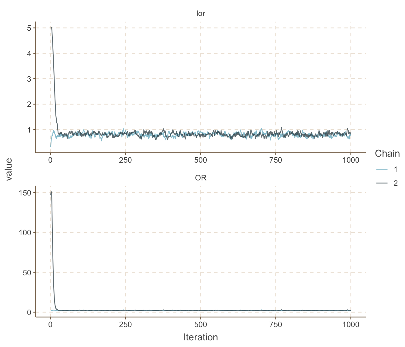
圖 100.12: Density plots for parameters prediction in smoking and cancer case-control study.
## Potential scale reduction factors:
##
##          Point est. Upper C.I.
## OR             1.01       1.06
## deviance       1.03       1.09
## lor            1.02       1.07
##
## Multivariate psrf
##
## 1.03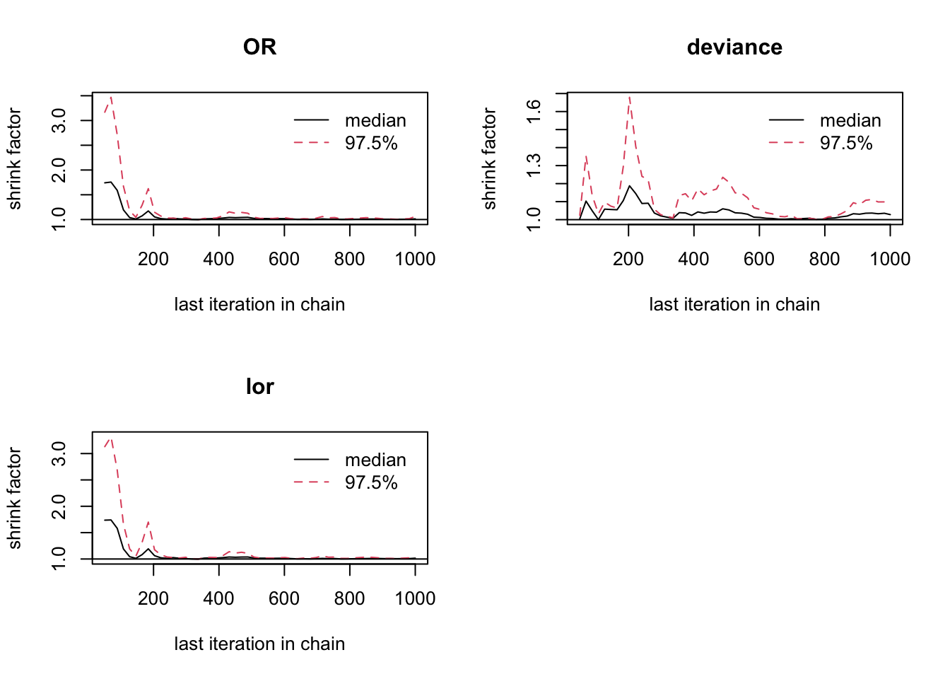
圖 100.13: Gelman-Rubin convergence statistic for smoking and cancer cohort study.
jagsModel <- jags(data = Dat,
                  model.file = paste(bugpath,
                                  "/backupfiles/case-control-model.txt",
                                  sep = ""),
                    parameters.to.save = c("OR", "lor"),
                     n.iter = 26000,
                     n.chains = 2,
                     inits = inits,
                     n.burnin = 1000,
                     n.thin = 1,
                    progress.bar = "none")
## Compiling model graph
## Resolving undeclared variables
## Allocating nodes
## Graph information:
## Observed stochastic nodes: 2
## Unobserved stochastic nodes: 2
## Total graph size: 13
##
## Initializing model## Inference for Bugs model at "/Users/chaoimacmini/Downloads/LSHTMlearningnote/backupfiles/case-control-model.txt", fit using jags,
## 2 chains, each with 26000 iterations (first 1000 discarded)
## n.sims = 50000 iterations saved
## mu.vect sd.vect 2.5% 25% 50% 75% 97.5% Rhat n.eff
## OR 2.280 1.628 1.925 2.131 2.250 2.373 2.635 1.054 28000
## lor 0.812 0.099 0.655 0.756 0.811 0.864 0.969 1.002 50000
## deviance 18.199 52.611 15.381 15.909 16.742 18.138 22.836 1.039 26000
##
## For each parameter, n.eff is a crude measure of effective sample size,
## and Rhat is the potential scale reduction factor (at convergence, Rhat=1).
##
## DIC info (using the rule, pD = var(deviance)/2)
## pD = 1383.8 and DIC = 1402.0
## DIC is an estimate of expected predictive error (lower deviance is better).100.5.2.3 聯合模型 joint model
把兩個甚至多個不同的研究獲得的數據聯合起來的方法主要有兩種,一是使用其中一個或者多個的研究結果作爲有信息的先驗概率分布,放到之後的研究模型中去,二是把多個不同的研究用共同的位置變量聯通起來 (link sub-models for different data sources through common parameter(s))。在這個吸煙和癌症的研究話題中,我們發現隊列研究,和病例對照研究兩者之間有共同的未知變量-比值比 (OR),如果這個比值比有這相同的含義,那麼我們可以通過它把兩個獨立的研究連接起來。
我們提供一個聯合模型的例子如下(保存爲jointmodel.txt):
# Joint model

model{
        # cohort sub-model
        Y0c ~ dbin(r0, X0c) # data model for non-smokers
        logit(r0) <- lr0
        Y1c ~ dbin(r1, X1c) # data model for smokers
        logit(r1) <- lr1
        lr1 <- lr0 + lor # lor is log(OR)
        # prior for cohort sub-model
        lr0 ~ dnorm(0, 0.3) # prior for logOdds of nonsmokers

        # case-control sub-model
        X0cc ~ dbin(p0, Y0cc) # data model for non-cancer controls
        logit(p0) <- lp0
        X1cc ~ dbin(p1, Y1cc) # data model for cancer cases
        logit(p1) <- lp1
        lp1 <- lp0 + lor # lor is log(OR)
        # prior for case-control sub-model
        lp0 ~ dnorm(0, 0.3) # prior for logOdds of exposure for controls

        # Common code
        lor ~ dnorm(0, 0.33) # prior for common log(OR)
        OR <- exp(lor) # comparison statistic
}把兩個獨立研究的數據合並成爲一個(保存成爲dataforjoint.txt):
list(X0c  = 2000,
         Y0c  = 100,
         X1c  = 1000,
         Y1c  = 150,
         X0cc = 800,
         Y0cc = 2000,
         X1cc = 600,
         Y1cc = 1000
)
接下來是對聯合模型的擬合及對OR值事後樣本的採集過程:
# Data file for the model
Dat <- list(X0c  = 2000,
                Y0c  = 100,
                X1c  = 1000,
                Y1c  = 150,
                X0cc = 800,
                Y0cc = 2000,
                X1cc = 600,
                Y1cc = 1000)

# initial values for the model
# the choice is arbitrary

inits <- list(
 list(lr0 = -1, lp0 = -2, lor = 0),
 list(lr0 = -5, lp0 = 2, lor = 5)
)

# fit the model in jags
jagsModel <- jags(data = Dat,
                  model.file = paste(bugpath,
                                  "/backupfiles/jointmodel.txt",
                                  sep = ""),
                    parameters.to.save = c("OR", "lor"),
                     n.iter = 1000,
                     n.chains = 2,
                     inits = inits,
                     n.burnin = 0,
                     n.thin = 1,
                    progress.bar = "none")
## Compiling model graph
## Resolving undeclared variables
## Allocating nodes
## Graph information:
## Observed stochastic nodes: 4
## Unobserved stochastic nodes: 3
## Total graph size: 21
##
## Initializing model# Show the trace plot
Simulated <- coda::as.mcmc(jagsModel)
ggSample <- ggs(Simulated)
ggSample %>%
filter(Parameter %in% c("OR", "lor")) %>%
ggs_traceplot()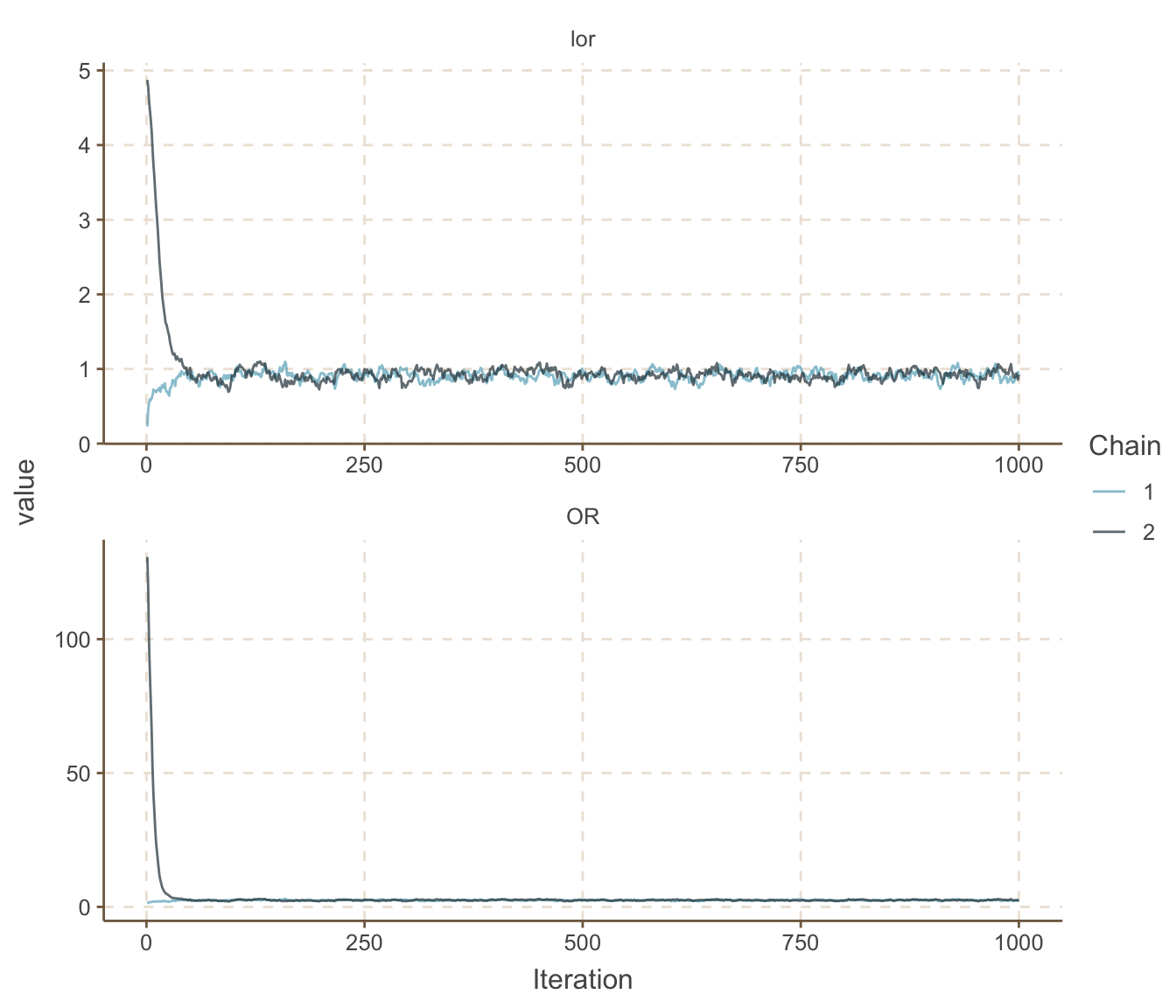
圖 100.14: Density plots for parameters prediction in smoking and cancer joint model.
## Potential scale reduction factors:
##
##          Point est. Upper C.I.
## OR             1.01       1.03
## deviance       1.02       1.03
## lor            1.01       1.04
##
## Multivariate psrf
##
## 1.01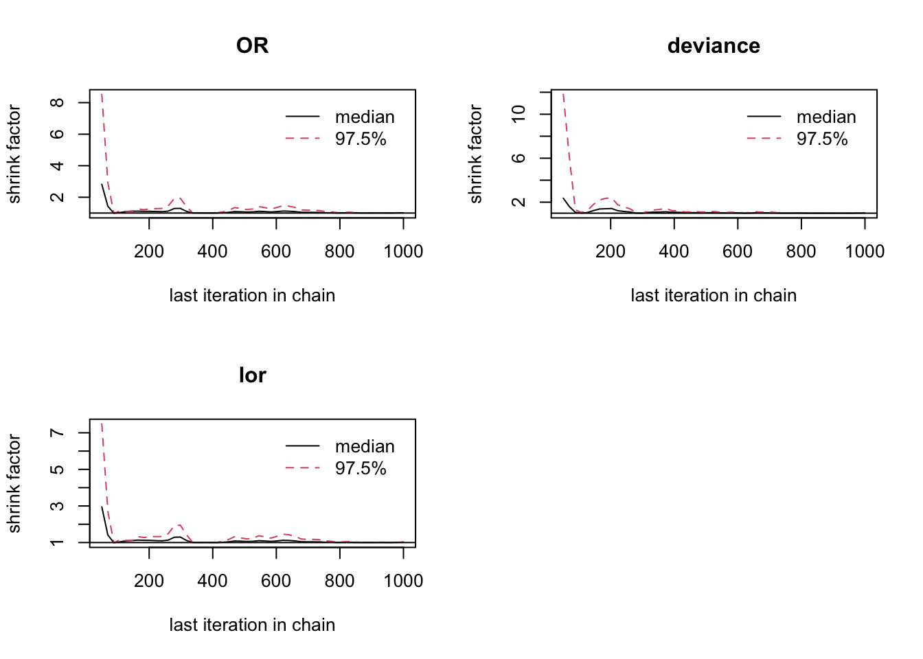
圖 100.15: Gelman-Rubin convergence statistic for smoking and cancer cohort study.
jagsModel <- jags(data = Dat,
                  model.file = paste(bugpath,
                                  "/backupfiles/jointmodel.txt",
                                  sep = ""),
                    parameters.to.save = c("OR", "lor"),
                     n.iter = 26000,
                     n.chains = 2,
                     inits = inits,
                     n.burnin = 1000,
                     n.thin = 1,
                    progress.bar = "none")
## Compiling model graph
## Resolving undeclared variables
## Allocating nodes
## Graph information:
## Observed stochastic nodes: 4
## Unobserved stochastic nodes: 3
## Total graph size: 21
##
## Initializing model## Inference for Bugs model at "/Users/chaoimacmini/Downloads/LSHTMlearningnote/backupfiles/jointmodel.txt", fit using jags,
## 2 chains, each with 26000 iterations (first 1000 discarded)
## n.sims = 50000 iterations saved
## mu.vect sd.vect 2.5% 25% 50% 75% 97.5% Rhat n.eff
## OR 2.509 1.099 2.178 2.376 2.487 2.603 2.842 1.065 15000
## lor 0.912 0.086 0.779 0.865 0.911 0.957 1.045 1.006 50000
## deviance 38.958 57.785 35.151 36.168 37.317 39.067 44.113 1.082 5000
##
## For each parameter, n.eff is a crude measure of effective sample size,
## and Rhat is the potential scale reduction factor (at convergence, Rhat=1).
##
## DIC info (using the rule, pD = var(deviance)/2)
## pD = 1669.3 and DIC = 1708.2
## DIC is an estimate of expected predictive error (lower deviance is better).可以看到,聯合模型給出的事後OR均值(2.513)是位於兩個獨立研究給出的OR均值(3.356, 2.273)的中間。但是它更加靠近病例對照研究的結果,暗示我們兩個研究中病例對照研究給出的信息量相對權重較大。另外,事後OR分布的標準差本身比兩個獨立研究估計的事後OR分布標準差都要小,說明充分利用兩個研究的數據時,事後估計的精確度得到了提升。精確度提升的原因很容易理解,因爲聯合模型把二者獲得的數據都包含了進來,信息量比兩個獨立研究都要大。
100.5.2.4 你是否能證明兩個研究的比值比是相同的?
對於隊列研究來說,我們估計其比值比所用的表格可以寫作:
| Cancer | ||||
|---|---|---|---|---|
| Y | N | |||
| Smoking | Y | S | ||
| N | NS | |||
| C | NC |
那麼這個研究中的比值比計算式就是:
\[ \text{OR}_{\text{cohort}} = \frac{\text{Pr}(C|S)\times\text{Pr}(NC|NS)}{\text{Pr}(C|NS)\times\text{Pr}(NC|S)} \]
對於病例對照研究來說,其比值比估計時使用的表格是:
| Smoking | ||||
|---|---|---|---|---|
| Y | N | |||
| Cancer | Y | C | ||
| N | NC | |||
| S | NS |
其比值比的計算式可以寫作:
\[ \text{OR}_{\text{case-control}} = \frac{\text{Pr}(S|C)\times\text{Pr}(NS|NC)}{\text{Pr}(S|NC)\times\text{Pr}(NS|C)} \]
可以證明兩者相同(反復使用貝葉斯定理):
\[ \begin{aligned} \text{OR}_{\text{cohort}} & = \frac{\text{Pr}(C|S)\times\text{Pr}(NC|NS)}{\text{Pr}(C|NS)\times\text{Pr}(NC|S)} \\ & = \frac{\frac{\text{Pr}(S|C)\text{Pr}(C)}{\text{Pr}(S)}\times\frac{\text{Pr}(NS|NC)\text{Pr}(NC)}{\text{Pr}(NS)}}{\frac{\text{Pr}(NS|C)\text{Pr}(C)}{\text{Pr}(NS)}\times\frac{\text{Pr}(S|NC)\text{Pr}(NC)}{\text{Pr}(S)}} \\ & = \frac{\text{Pr}(S|C)\times\text{Pr}(NS|NC)}{\text{Pr}(S|NC)\times\text{Pr}(NS|C)} \\ & = \text{OR}_{\text{case-control}} \end{aligned} \]