第 94 章 貝葉斯生存分析 Bayesian Survival Analysis
我們使用相同的白血病患者數據來展示分析代碼和結果:
Example 94.1 給白血病患者數據套用 Cox 比例風險回歸模型 在這個數據中,42名白血病患者中各有21人分別在治療和對照組。研究者關心的事件是病情的緩解 (remission)。追蹤時間是從白血病診斷時起,單位是週數。那麼暴露變量就是被分配到治療組與否,其中被分配到對照組的患者的風險度被認爲是基線風險度 (baseline hazard)。於是這個模型其實可以簡單描述成:
\[ \begin{cases} h_0(t) & 對照組 \text{ control group} \\ h_0(t) e^\beta & 治療組 \text{ treatment group} \end{cases} \]
使用偏似然法計算該模型的參數我們獲得對數風險度比 (log hazard ratio) 的估計值 \(\hat\beta = -1.51\),其對應的標準誤是 \(0.410\),95% 信賴區間是 (-2.31, -0.71)。於是相應的,風險度比 \(\exp \hat\beta = 0.22\),95% 信賴區間是 \((0.10, 0.49)\)。
該模型用 Stata 計算的過程如下
##
## . infile group weeks remission using https://data.princeton.edu/wws509/datasets
## > /gehan.raw
## host not found
## r(631);
##
## . label define group 1 "control" 2 "treated"
##
## . label values group group
## no variables defined
## r(111);
##
## . stset weeks, failure(remission)
## variable weeks not found
## r(111);
##
## . stcox group
## variable group not found
## r(111);
##
## . stcox group, nohr
## variable group not found
## r(111);
##
## .
該模型用 R 計算的過程如下
gehan <- read.table("https://data.princeton.edu/wws509/datasets/gehan.raw",
                    header =  FALSE, sep ="",
                    col.names = c( "group", "weeks", "remission"))

cox.model <- coxph(Surv(time = weeks, event = remission) ~ as.factor(group),
                     data = gehan, method = "breslow")
summary(cox.model)
## Call:
## coxph(formula = Surv(time = weeks, event = remission) ~ as.factor(group),
## data = gehan, method = "breslow")
##
## n= 42, number of events= 30
##
## coef exp(coef) se(coef) z Pr(>|z|)
## as.factor(group)2 -1.50919 0.22109 0.40956 -3.6849 0.0002288 ***
## ---
## Signif. codes: 0 '***' 0.001 '**' 0.01 '*' 0.05 '.' 0.1 ' ' 1
##
## exp(coef) exp(-coef) lower .95 upper .95
## as.factor(group)2 0.22109 4.5231 0.099071 0.49339
##
## Concordance= 0.69 (se = 0.041 )
## Likelihood ratio test= 15.21 on 1 df, p=0.0001
## Wald test = 13.58 on 1 df, p=0.0002
## Score (logrank) test = 15.93 on 1 df, p=7e-05相同的模型如果使用 brms 通過 Stan 運行貝葉斯模型的話是這樣子的:
gehan <- gehan %>%
  mutate( remission1 = 1 - remission ) %>%
  mutate( Group = as.factor(group) )

fitCox1002 <-
  brm(data = gehan,
      family = brmsfamily("cox"),
      weeks | cens(remission1) ~ 1 + Group,
      iter = 4000, warmup = 1500, chains = 4, cores = 4,
      seed = 14)
saveRDS(fitCox1002, "../Stanfits/Cox1002.rds")
Check the summary for fitCox1002.
##  Family: cox
##   Links: mu = log
## Formula: weeks | cens(remission1) ~ 1 + Group
##    Data: gehan (Number of observations: 42)
##   Draws: 4 chains, each with iter = 4000; warmup = 1500; thin = 1;
##          total post-warmup draws = 10000
##
## Population-Level Effects:
##           Estimate Est.Error l-95% CI u-95% CI Rhat Bulk_ESS Tail_ESS
## Intercept     1.57      0.33     0.96     2.24 1.00     6732     6706
## Group2       -1.68      0.43    -2.55    -0.88 1.00     8812     6939
##
## Draws were sampled using sampling(NUTS). For each parameter, Bulk_ESS
## and Tail_ESS are effective sample size measures, and Rhat is the potential
## scale reduction factor on split chains (at convergence, Rhat = 1).
計算對應的貝葉斯事後危險度比 Hazard Ratio
## Warning: Method 'posterior_samples' is deprecated. Please see ?as_draws for recommended
## alternatives.
post %>%
transmute(`hazard ratio` = exp(b_Group2)) %>%
summarise(median = median(`hazard ratio`),
sd = sd(`hazard ratio`),
ll = quantile(`hazard ratio`, probs = .025),
ul = quantile(`hazard ratio`, probs = .975)) %>%
mutate_all(round, digits = 4)## median sd ll ul
## 1 0.19 0.0875 0.0781 0.4154繪製貝葉斯方法獲得的事後分佈概率密度函數 (Why not glance at the full posterior?):
post %>%
  transmute(`hazard ratio` = exp(b_Group2)) %>%
  ggplot(aes(x = `hazard ratio`, y = 0)) +
  geom_vline(xintercept = 1, color = "white") +
  stat_halfeye(.width = c(.5, .95)) +
  scale_y_continuous(NULL, breaks = NULL) +
  xlab("hazard ratio for Group2 vs Group1") +
  theme(panel.grid = element_blank())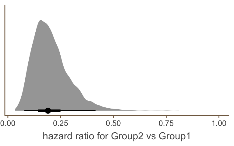
圖 94.1: The full posterior distribution of the hazard ratio from model fitCox1002
從已經運行好的模型中調取 brms 自動爲我們生成的 Stan 代碼:
## // generated with brms 2.15.0
## functions {
##   /* distribution functions of the Cox proportional hazards model
##    * parameterize hazard(t) = baseline(t) * mu
##    * so that higher values of 'mu' imply lower survival times
##    * Args:
##    *   y: the response value; currently ignored as the relevant
##    *     information is passed via 'bhaz' and 'cbhaz'
##    *   mu: positive location parameter
##    *   bhaz: baseline hazard
##    *   cbhaz: cumulative baseline hazard
##    */
##   real cox_lhaz(real y, real mu, real bhaz, real cbhaz) {
##     return log(bhaz) + log(mu);
##   }
##   real cox_lccdf(real y, real mu, real bhaz, real cbhaz) {
##     // equivalent to the log survival function
##     return - cbhaz * mu;
##   }
##   real cox_lcdf(real y, real mu, real bhaz, real cbhaz) {
##     return log1m_exp(cox_lccdf(y | mu, bhaz, cbhaz));
##   }
##   real cox_lpdf(real y, real mu, real bhaz, real cbhaz) {
##     return cox_lhaz(y, mu, bhaz, cbhaz) + cox_lccdf(y | mu, bhaz, cbhaz);
##   }
##   // Distribution functions of the Cox model in log parameterization
##   real cox_log_lhaz(real y, real log_mu, real bhaz, real cbhaz) {
##     return log(bhaz) + log_mu;
##   }
##   real cox_log_lccdf(real y, real log_mu, real bhaz, real cbhaz) {
##     return - cbhaz * exp(log_mu);
##   }
##   real cox_log_lcdf(real y, real log_mu, real bhaz, real cbhaz) {
##     return log1m_exp(cox_log_lccdf(y | log_mu, bhaz, cbhaz));
##   }
##   real cox_log_lpdf(real y, real log_mu, real bhaz, real cbhaz) {
##     return cox_log_lhaz(y, log_mu, bhaz, cbhaz) +
##            cox_log_lccdf(y | log_mu, bhaz, cbhaz);
##   }
## }
## data {
##   int<lower=1> N;  // total number of observations
##   vector[N] Y;  // response variable
##   int<lower=-1,upper=2> cens[N];  // indicates censoring
##   int<lower=1> K;  // number of population-level effects
##   matrix[N, K] X;  // population-level design matrix
##   // data for flexible baseline functions
##   int Kbhaz;  // number of basis functions
##   // design matrix of the baseline function
##   matrix[N, Kbhaz] Zbhaz;
##   // design matrix of the cumulative baseline function
##   matrix[N, Kbhaz] Zcbhaz;
##   // a-priori concentration vector of baseline coefficients
##   vector<lower=0>[Kbhaz] con_sbhaz;
##   int prior_only;  // should the likelihood be ignored?
## }
## transformed data {
##   int Kc = K - 1;
##   matrix[N, Kc] Xc;  // centered version of X without an intercept
##   vector[Kc] means_X;  // column means of X before centering
##   for (i in 2:K) {
##     means_X[i - 1] = mean(X[, i]);
##     Xc[, i - 1] = X[, i] - means_X[i - 1];
##   }
## }
## parameters {
##   vector[Kc] b;  // population-level effects
##   real Intercept;  // temporary intercept for centered predictors
##   simplex[Kbhaz] sbhaz;  // baseline coefficients
## }
## transformed parameters {
## }
## model {
##   // likelihood including constants
##   if (!prior_only) {
##     // compute values of baseline function
##     vector[N] bhaz = Zbhaz * sbhaz;
##     // compute values of cumulative baseline function
##     vector[N] cbhaz = Zcbhaz * sbhaz;
##     // initialize linear predictor term
##     vector[N] mu = Intercept + Xc * b;
##     for (n in 1:N) {
##     // special treatment of censored data
##       if (cens[n] == 0) {
##         target += cox_log_lpdf(Y[n] | mu[n], bhaz[n], cbhaz[n]);
##       } else if (cens[n] == 1) {
##         target += cox_log_lccdf(Y[n] | mu[n], bhaz[n], cbhaz[n]);
##       } else if (cens[n] == -1) {
##         target += cox_log_lcdf(Y[n] | mu[n], bhaz[n], cbhaz[n]);
##       }
##     }
##   }
##   // priors including constants
##   target += student_t_lpdf(Intercept | 3, 2.4, 2.5);
##   target += dirichlet_lpdf(sbhaz | con_sbhaz);
## }
## generated quantities {
##   // actual population-level intercept
##   real b_Intercept = Intercept - dot_product(means_X, b);
## }