第 81 章 主成分分析 Principal Component Analysis
- A big computer, a complex algorithm and a long time does not equal science.
- Robert Gentleman
81.1 數據有相關性時產生的問題
假設我們有 \(n\) 個研究對象作爲樣本,我們從這些對象身上採集儘可能多的數據,假設我們一共收集了 \(p\) 個不同的變量。那麼這個數據的維度 (dimension) 是 \(n \times p\)。
如果說,我們在這個樣本中獲取到的 \(p\) 個變量中,有一些是相互有依存性的,或者說相關的 (correlated)。我們有沒有辦法描述並展示這些具有相關性的變量在這個數據中扮演的角色,並且保留整個數據本身的變化特徵 (variability)?
Edgeworth (1891) 最早試圖用下面的方程來歸納一組從男性樣本身上測量獲得的存在相關性的變量:身高(H),前臂長(F),腿長(L):
\[ \begin{aligned} Y_1 & = 0.16H + 0.51F + 0.39L \\ Y_2 & = -0.17H + 0.69F + 0.09L \\ Y_3 & = -0.15H + 0.25F + 0.52L \end{aligned} \]
這恐怕是最早嘗試將一組有相關性的身體測量數據整理成”不相關”的三個新變量,作爲男性身體測量指標,用於描述樣本個體的身體結構的過程。
下圖 81.1 中展示的兩個變量,\(x_1\) 和 \(x_2\) 分別是身高和體重。
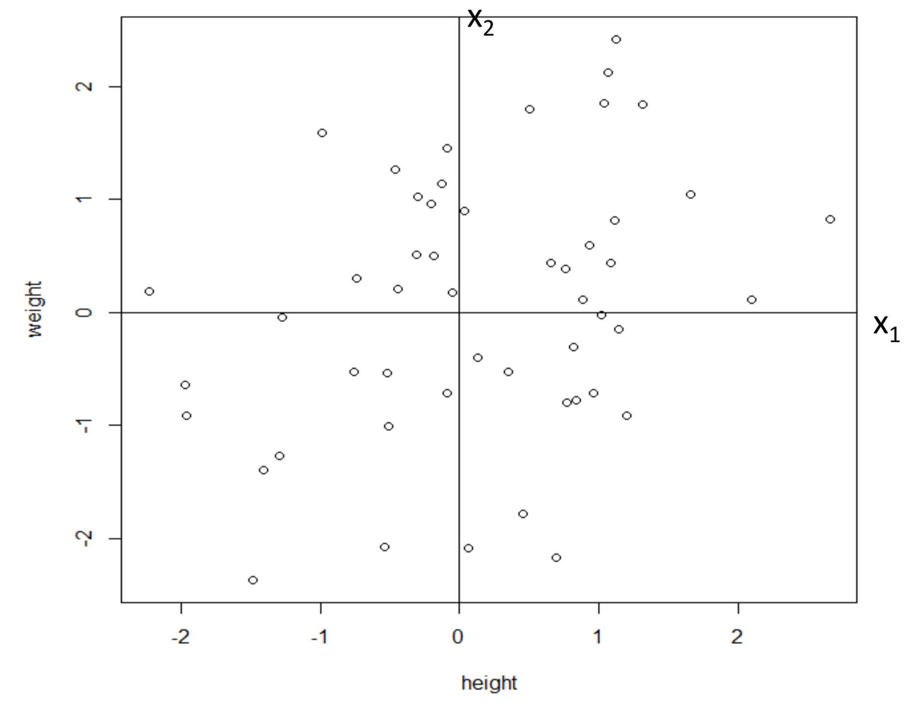
圖 81.1: Standardised data of height and weight
變量經過標準化處理之後,均值 \(\mu = 0\),方差 \(\sigma^2 =1\)。如果此時已知身高和體重之間的協方差 (covariance, 概念參考 Section 8.1) 是 \(0.3\)。
那麼,可以推導證明的是,他們的相關係數 (correlation, 概念參考 Section 8.2) 是:
\[ \begin{aligned} Corr(X_1,X_2) & = \frac{Cov(X_1,X_2)}{SD(X_1)SD(X_2)} \\ & =\frac{Cov(X_1,X_2)}{\sqrt{Var(X_1)Var(X_2)}}\\ & = Cov(X_1,X_2) \\ & = 0.3 \end{aligned} \]
以 \(x_2\) (體重) 爲結果變量,\(X_1\) (身高) 爲單一解釋變量的線性回歸模型的回歸係數 (regression coefficient \(\hat\beta\), 概念參考 Section 28.2) 是:
\[ \begin{aligned} \hat\beta & = \frac{S_{x_1x_2}}{SS_{x_1x_2}} \\ & = \frac{CV_{x_1x_2}}{SD_{x_1}^2} \\ & = 0.3 \end{aligned} \]
如果我們有另外一個座標系如下圖 81.2,從原先的座標系進行了一定角度的旋轉獲得 \(y_1, y_2\)。你會認爲哪個座標系更適合這個標準化之後身高體重的數據呢?
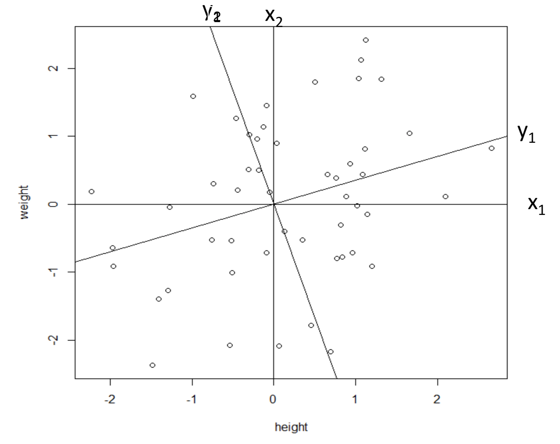
圖 81.2: Standardised data of height and weight, with a new reference system (y_1, y_2)
其實原先 \(x_1, x_2\) 座標系之間存在一定的相關性,我們希望經過旋轉之後的新座標系 \(y_1, y_2\) 之間是垂直的 (orthogonal),這一數學上的概念被翻譯成爲統計學的語言就是,希望旋轉之後的新座標(變量)之間沒有相關性 (uncorrelated)。爲了消滅變量之間的相關性,我們要尋找到一個旋轉的角度 \(\theta\),使得所有數據的點 \(P_j\) 到新的座標軸 \(y_1\) 之間的垂直距離(perpendicualr) \(P_jP_j^\prime\) 之和最小 (minimise the distances between points and the reference axes)。如圖 81.3 顯示的那樣,從原點到每個數據點 \(P_j\) 之間的距離 \(OP_j\) 其實是固定不變的。我們希望找到新的座標使得 \(P_jP_j^\prime\) 的距離最短。其中 \(OP_j^\prime\) 就是數據點在新座標軸上投影的長度。
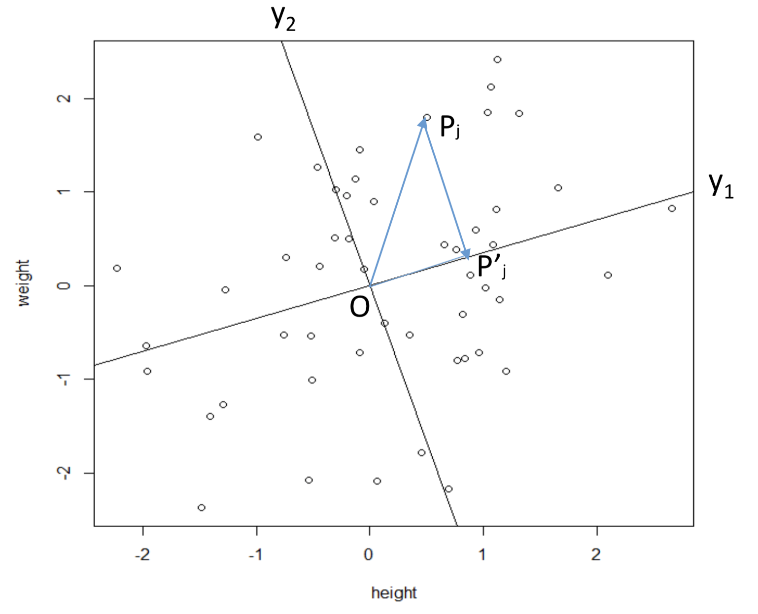
圖 81.3: Minimise the distance between the points and the reference axes.
根據勾股定理 (Pythagorean theorem)。圖 81.3 中直角三角形的三邊的長度關係可以描述爲:
\[ (OP_j)^2 = (P_jP_j^\prime)^2 + (OP_j^\prime)^2 \]
把勾股定理應用到全部的數據點上的話,我們會得到一個關於所有數據點到新的座標軸距離,以及原點之間距離的方程:
\[ \begin{equation} \sum_j (OP_j)^2 = \sum_j(P_jP_j^\prime)^2 + \sum_j(OP_j^\prime)^2 \end{equation} \tag{81.1} \]
81.2 最大化方差等價於最大化數據點到新座標軸“投影(projection)”的長度
把等式 (81.1) 兩邊同時除以數據樣本量,我們獲得等式 (81.2):
\[ \begin{equation} \sum_j (OP_j)^2/n = \sum_j(P_jP_j^\prime)^2/n + \sum_j(OP_j^\prime)^2/n \end{equation} \tag{81.2} \]
其中值得注意的是,等式 (81.2) 左邊的部分 \(\sum_j (OP_j)^2/n\) 對於一個樣本來說是固定不變的 (constant)。於是,等式右邊的部分,當我們的目標是最小化 \(\sum_j(P_jP_j^\prime)^2/n\) 垂線 (perpendicular) 長度之和時,就等價於把數據點在新座標軸上的投影之和 \(\sum_j(OP_j^\prime)^2/n\) 最大化。說白了,數據點在新座標軸上的投影,就是新座標軸上的變量大小。所以,旋轉座標軸之後,我們希望產生的新變量 \(y_1,y_2\) 的方差取最大值(maximising the variance of the new data \(\sum_j(OP_j^\prime)^2/n\))。利用三角函數(假設座標軸的旋轉角度是\(\theta\)),你很容易就能得到新座標軸上新變量的值:
\[ \begin{equation} \begin{aligned} y_1 & = x_1\cos\theta + x_2\sin\theta \\ y_2 & = -x_1\sin\theta + x_2\cos\theta \end{aligned} \end{equation} \tag{81.3} \]
證明
如圖 81.4 所示,設座標軸 \(X_1,X_2\) 逆時針旋轉角度爲 \(\theta\),設新座標爲 \((y_1, y_2)\),且原點於點 \(P_j (x_1, x_2)\) 之間的連線 \(OP_j\) 長度爲 \(r\),\(OP_j\) 和新座標軸 \(y_1\) 之間的角度爲 \(\alpha\)。
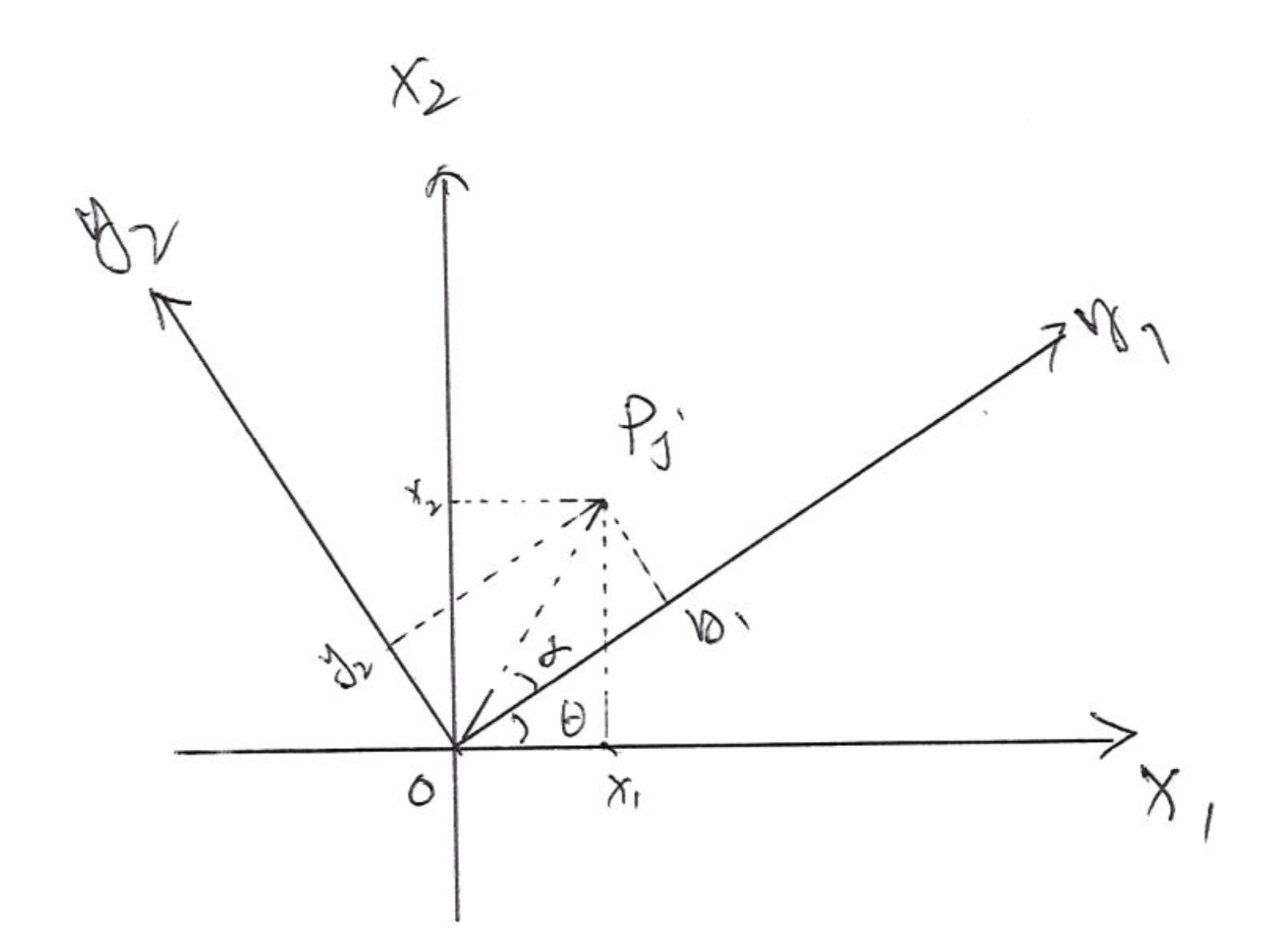
圖 81.4: Rotation of the coordinates, and the new variables calculation.
\[ \begin{aligned} (OP_j)^2 & = x_1^2 + x_2^2 = y_1^2 + y_2^2 \\ & = r^2 \\ \because x_1 & = r\times\cos(\alpha +\theta) \\ x_2 & = r\times\sin(\alpha + \theta) \\ y_1 & = r\times\cos(\alpha) \\ y_2 & = r\times\sin(\alpha) \\ \therefore x_1 & = r[\cos\alpha\cos\theta - \sin\alpha\sin\theta] \\ & = y_1\cos\theta - y_2\sin\theta \\ x_2 & = r[\sin\alpha\cos\theta + \cos\alpha\sin\theta] \\ & = y_2\cos\theta+y_1\sin\theta \\ \Rightarrow x_1\cos\theta & = y_1\cos^2\theta -y_2 \sin\theta\cos\theta \\ x_2\sin\theta & = y_2\cos\theta\sin\theta + y_1\sin^2\theta \\ \textbf{Sum the}& \textbf{ above two equations} \\ \Rightarrow y_1 & = \frac{x_1\cos\theta + x_2 \sin\theta}{(\cos^2\theta + \sin^2\theta)} \\ y_1 & = x_1\cos\theta + x_2 \sin\theta \\ \textbf{Similarly}& \\ \Rightarrow x_1\sin\theta & = y_1\cos\theta\sin\theta -y_2 \sin^2\theta \\ x_2\cos\theta & = y_2\cos^2\theta + y_1\sin\theta\cos\theta \\ \textbf{Take substraction}& \textbf{ between the above two equations} \\ \Rightarrow y_2 & = \frac{-x_1\sin\theta + x_2\cos\theta}{(\cos^2\theta + \sin^2\theta)} \\ y_2 & = -x_1\sin\theta + x_2\cos\theta \end{aligned} \]
\(y_1, y_2\)就是旋轉後新的座標軸的變量。在這個簡單實例中,我們從原始數據 \(x_1, x_2\) 經過旋轉,獲得新的數據 \(y_1, y_2\),他們二者之間其實只是經過了線性轉換 (linear transformation)。一般地,我們如果要給原始數據矩陣 (維度 \(n\times p\))進行座標軸的數據轉換,只需要給原始數據矩陣乘以一個正方形的投影矩陣 \(\mathbf{P}\) (projection matrix) (維度 \(p\times p\)) (\(p\) 是變量的個數)即可。
當變量只有兩個 \((p =2)\) 時,我們很容易使用一個平面圖來理解這個轉換過程其實就是對座標軸進行幾何旋轉的過程,這時候的投影矩陣是:
\[ \left[ \begin{array} \cos\cos\theta & \sin\theta \\ -\sin\theta & \cos\theta \end{array} \right] \tag{81.4} \]
經過旋轉之後獲得的新變量 \(y_1, y_2\) 被叫做主成分 (principal components)。主成分有什麼特徵呢?如圖 81.5 所表示的那樣,當兩個原始變量 \(x_1, x_2\) 之間相關係數很高,由於已知方差總和不變 \(\text{Var}(x_1)+\text{Var}(x_2) = \text{Var}(y_1) + \text{Var}(y_2)\),座標旋轉之後的第一個主成分 \(y_1\),將會擁有原始數據 \(x_1, x_2\) 的方差 (variance) 中的絕大部分。那麼理論上,我們就完成了保留數據本身的整體方差,但是把大部分方差歸納到第一個主成分中去的過程。所以,當對樣本測量了很多很多的變量的時候,我們會發現很多變量之間存在內部相關性,於是我們可以通過主成分分析來留下幾個能解釋整體數據的最主要的成分,並且保留數據的整體信息,也就是整體的方差,這是一個把數據降維 (dimension reduction) 的過程,去除掉那些冗餘的不需要的變量 (redundancy removed)。
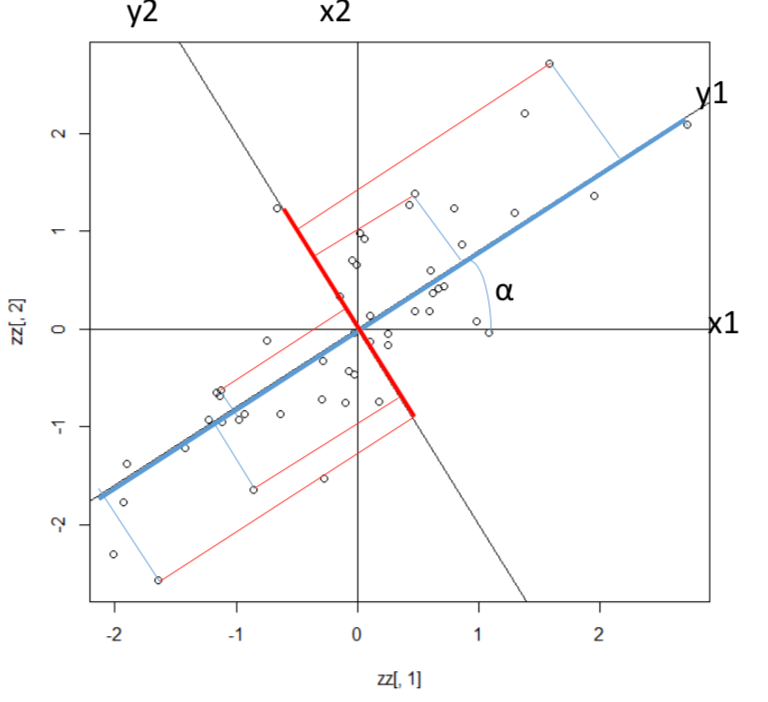
圖 81.5: Variance of the new axis/prin
所以,PCA的過程可以描述如下:
數據如果有 \(p\) 個存在內部相關性的連續型變量 \(x_1, x_2, \dots, x_p\),那麼一定存在 \(p\) 個相互獨立的變量 (principal components),滿足下面的條件:
\(p\) 個相互獨立的變量分別都是原始變量 \(x_1, x_2, \dots, x_p\) 的線性轉換: \[ \begin{aligned} y_1 & = a_{11}x_1 + a_{12}x_2 + \cdots + a_{1p}x_p \\ y_2 & = a_{21}x_1 + a_{22}x_2 + \cdots + a_{2p}x_p \\ \vdots & \\ y_p & = a_{p1}x_1 + a_{p2}x_2 + \cdots + a_{pp}x_p \\ \end{aligned} \]
這 \(p\) 個相互獨立的變量通過最大化它們對數據整體方差的貢獻獲得。
這 \(p\) 個相互獨立的變量被叫做這個數據的主成分變量。
這些主成分變量之間相互獨立 (uncorrelated),並且按照他們各自對數據總體方差的貢獻度從大到小排列 (the principal components are uncorrelated and are ordered by the amount of the total system variability that they explain):
\[ \text{Cov}(y_j, y_k) = 0 \text{ for any } j, k \in [1, p] \\ \text{Var}(y_1) \geqslant \text{Var}(y_2) \geqslant \text{Var}(y_3) \geqslant \dots \geqslant \text{Var}(y_p) \]
81.3 數學推導
如果,
- \(\textbf{S}\) 是數據的方差協方差矩陣 (variance, covriance matrix);
- \(\textbf{P}\) 是直角投影矩陣 (orthogonal projection matrix),該矩陣的每一列,是旋轉之後的新變量的座標,也就是主成分變量,它們又被叫做特徵向量 (eigenvectors);
- \(\bf{\Lambda}\) 是一個對角矩陣 (diagonal matrix),它的對角線上是每個主成分變量的方差,它們又被叫做特徵值 (eigenvalues)。特徵值常常又被叫做慣性 (inertia),特徵值從對角線左上角起往右下角是從大到小排列,每一個特徵值是每個特徵向量的方差,也就是數據整體方差投射在這個主成分變量上的慣性,可以理解爲該主成分能夠解釋多少整個數據的方差 (explained variance)。
Theorem 81.1 (Spectral decomposition) 根據譜定理 Spectral decomposition:如果矩陣 \(\textbf{S}\) 是對稱的,它總是可以被分解爲: \[ \textbf{S} = \textbf{P}\bf{\Lambda}\textbf{P}^t \]
值得注意的是,首先,分解方差協方差矩陣的時候,並沒有任何統計學或者概率論上的前提條件;其次,這樣的矩陣分解不一定只用於方差協方差矩陣,你可以對任何對稱矩陣 (symmetrix matrix) 進行分解,它被叫做矩陣縮放 (matrix scaling);最後,其實數據矩陣本身不一定非要是連續型變量,也不一定要有相似的刻度/取值範圍 (same scale),如果你願意,對二分類變量或者是計數型變量,均可以進行主成分分析。但是,當變量之間的刻度相差巨大時,可能會產生一些意想不到的假象。所以,在實施主成分分析之前,通常的建議是對原始數據的變量進行標準化,或者直接用其相關係數矩陣 (correlation matrix)。
81.3.1 超越對稱矩陣:奇異值分解 (singular value decomposition, SVD)
主成分分析使用的矩陣分解方法,只能應用在方差協方差矩陣或者相關係數矩陣這樣的對稱的正方形矩陣。假如矩陣並非對稱,另一種矩陣分解方法叫做奇異值分解法 (singular value decomposition, SVD)。此時就可以直接應用在原始數據矩陣 \(\mathbf{X}_{n\times p}\) 本身,而不需要侷限於數據的方差協方差矩陣/相關係數矩陣:
\[ \mathbf{X}_{n\times p} = \mathbf{U}_{n\times n}\bf{\Sigma}_{n \times p} \mathbf{W}_{p\times p}^t \]
其中,
- \(\mathbf{U}_{n\times n}\) 是含有左奇異向量 (left singular vectors) 的矩陣;
- \(\Sigma_{n \times p}\) 是含有奇異值 (singular values)的矩陣;
- \(\mathbf{W}_{p\times p}\) 則是含有右奇異向量 (right singular vectors) 的矩陣。
所以你看到任意的形狀都可以被分解,此時分解出來的 \(\mathbf{U}_{n\times n}\) 和 \(\mathbf{W}_{p\times p}\) 是形狀維度不同的正方形矩陣。
另外,根據這樣的分解我們可以推導:
\[ \begin{aligned} \mathbf{X}^t \mathbf{X} & = \mathbf{W}\bf{\Sigma}\mathbf{U}^t\times\mathbf{U}\bf{\Sigma}\mathbf{W}^t \\ & = \mathbf{W}\bf{\Sigma}^2\mathbf{W}^t \\ \Rightarrow \bf{\Sigma}^2 & = \bf{\Lambda} \end{aligned} \]
所以,\(\bf{\Sigma}^2 = \bf{\Lambda}\) ,也就是說在奇異值分解中獲得的中間矩陣 \(\bf{\Sigma}_{n \times p}\),它對角線上的數值的平方,就是每個原始變量的方差,或者說它們本身是原始數據的標準差。奇異值分解矩陣的方法最常見被用於實施對應分析 (Correspondence Analysis)。
81.4 主成分分析數據實例
橙汁數據,是邀請美食家對產自世界各地的六種品牌的橙汁進行一個一個的味道/品質描述,並給每個項目打分後彙總獲得的評價數據。你可以用下面的代碼下載這個數據並觀察每個描述的變量,且很容易觀察的到的是,這些變量之間並不完全獨立,有些變量可能和另一些變量相關:
| Odour.intensity | Odour.typicality | Pulpiness | Intensity.of.taste | Acidity | Bitterness | Sweetness | |
|---|---|---|---|---|---|---|---|
| Pampryl amb. | 2.82 | 2.53 | 1.66 | 3.46 | 3.15 | 2.97 | 2.60 |
| Tropicana amb. | 2.76 | 2.82 | 1.91 | 3.23 | 2.55 | 2.08 | 3.32 |
| Fruvita fr. | 2.83 | 2.88 | 4.00 | 3.45 | 2.42 | 1.76 | 3.38 |
| Joker amb. | 2.76 | 2.59 | 1.66 | 3.37 | 3.05 | 2.56 | 2.80 |
| Tropicana fr. | 3.20 | 3.02 | 3.69 | 3.12 | 2.33 | 1.97 | 3.34 |
| Pampryl fr. | 3.07 | 2.73 | 3.34 | 3.54 | 3.31 | 2.63 | 2.90 |
進行主成分分析在Stata只需要這樣一行代碼:
insheet using "http://factominer.free.fr/bookV2/orange.csv" , delimiter(";") clear
pca odour* pulp* intens* acid* bitter* sweetness, cor
你就會獲得十分直觀的結果:
Principal components/correlation                 Number of obs    =          6
                                                 Number of comp.  =          5
                                                 Trace            =          7
    Rotation: (unrotated = principal)            Rho              =     1.0000

    --------------------------------------------------------------------------
       Component |   Eigenvalue   Difference         Proportion   Cumulative
    -------------+------------------------------------------------------------
           Comp1 |      4.74369       3.4104             0.6777       0.6777
           Comp2 |      1.33329      .513448             0.1905       0.8681
           Comp3 |      .819842      .735818             0.1171       0.9853
           Comp4 |     .0840232     .0648702             0.0120       0.9973
           Comp5 |      .019153      .019153             0.0027       1.0000
           Comp6 |            0            0             0.0000       1.0000
           Comp7 |            0            .             0.0000       1.0000
    --------------------------------------------------------------------------

Principal components (eigenvectors)

    ------------------------------------------------------------------------------
        Variable |    Comp1     Comp2     Comp3     Comp4     Comp5 | Unexplained
    -------------+--------------------------------------------------+-------------
    odourinten~y |   0.2110    0.6534   -0.5174    0.0286    0.0310 |           0
    odourtypic~y |   0.4524    0.1162   -0.0646    0.2668    0.2952 |           0
       pulpiness |   0.3313    0.5340    0.3290   -0.3327   -0.2250 |           0
    intensityo~e |  -0.2984    0.3714    0.6910    0.0189    0.3456 |           0
         acidity |  -0.4191    0.3017   -0.0237    0.7065   -0.4106 |           0
      bitterness |  -0.4292    0.1628   -0.3152   -0.0974    0.6712 |           0
       sweetness |   0.4384   -0.1374    0.2061    0.5553    0.3503 |           0
    ------------------------------------------------------------------------------
根據方差協方差矩陣進行的主成分分析結果,我們發現主成分 6 和 7 可以忽略不計。相同的計算結果可以在R裏面通過方便的計算包 FactoMineR 來計算並用 factoextra 來實現其分析圖形的美觀展示:
# library(FactoMineR)
org.pca <- PCA(orange[, 1:7], ncp = 7, graph = FALSE)

# library(factoextra)
eig.val <- get_eigenvalue(org.pca)
eig.val # eigenvalue (variances of each principal components)
## eigenvalue variance.percent cumulative.variance.percent
## Dim.1 4.743692688 67.76703840 67.767038
## Dim.2 1.333289855 19.04699793 86.814036
## Dim.3 0.819841150 11.71201643 98.526053
## Dim.4 0.084023297 1.20033282 99.726386
## Dim.5 0.019153009 0.27361442 100.000000## [,1] [,2] [,3] [,4] [,5]
## [1,] 0.21100074 0.65340689 -0.517409852 0.028573070 0.030958154
## [2,] 0.45241413 0.11618305 -0.064606287 0.266760192 0.295222955
## [3,] 0.33132165 0.53403262 0.329025446 -0.332685134 -0.225026986
## [4,] -0.29836065 0.37144476 0.690990232 0.018942515 0.345597119
## [5,] -0.41905731 0.30166462 -0.023688451 0.706533003 -0.410644925
## [6,] -0.42917948 0.16282112 -0.315220908 -0.097425116 0.671196644
## [7,] 0.43840960 -0.13742859 0.206064224 0.555251136 0.350251763於是根據計算獲得的特徵值向量,我們可以寫下這5個主成分變量和原始變量之間的轉換關係方程:
\[ \begin{aligned} y_1 & = 0.2110x_1 + 0.4524x_2 + 0.3313x_3 - 0.2984x_4 - 0.4191x_5 - 0.4292x_6 + 0.4384x_7 \\ y_2 & = 0.6534x_1 + 0.1162x_2 + 0.5340x_3 + 0.3714x_4 + 0.3017x_5 + 0.1628x_6 - 0.1374x_7 \\ y_3 & =-0.5174x_1 - 0.0646x_2 + 0.3290x_3 + 0.6910x_4 - 0.0237x_5 - 0.3152x_6 + 0.2061x_7 \\ y_4 & = 0.0286x_1 + 0.2668x_2 - 0.3327x_3 + 0.0189x_4 + 0.7065x_5 - 0.0974x_6 + 0.5553x_7 \\ y_5 & = 0.0310x_1 + 0.2952x_2 - 0.2250x_3 + 0.3456x_4 - 0.4106x_5 + 0.6712x_6 + 0.3503x_7 \\ \end{aligned} \]
於是,解釋完了如何從原始數據變量根據計算獲得的特徵值向量轉換成爲新的變量之後,要面對的問題是,我們要保留多少主成分? 我們通常會使用圖 81.6 那樣的碎石圖 (Scree plot) 來輔助判斷。碎石圖通常縱軸是每個主成分能夠解釋的數據總體方差的百分比,然後橫軸是主成分的個數。所以我們會期待出現一個像手肘一樣的形狀提示應該在第幾個主成分的地方停下。通常在統計分析中,我們默認的準則是,至少保留的主成分個數要能夠解釋總體方差的 70%/80% 以上才較爲理想。Kaiser 準則 建議的是,最好保留下特徵值大於等於1(也就是標準化數據之後獲得的主成分變量方差大於等於1)的主成分變量。在我們的橙汁數據實例中,顯然保留前兩個主成分就已經能夠解釋 86.81% 的總體方差,我們認爲這是理想的主成分個數。
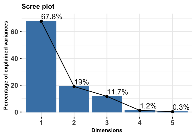
圖 81.6: Orange data: eigenvalues among all variances (varaince explained) by each dimension (principle component) provided by PCA
另外一種輔助的圖形是叫做分數圖 (score plot),又名個人圖 (graph of individuals),如果個體的變量特徵相近,他們會在圖中聚在較爲靠近的地方:
fviz_pca_ind(org.pca, pointsize = "cos2", pointshape = 21,
fill = "#E7B800", repel = TRUE, labelsize = 2) 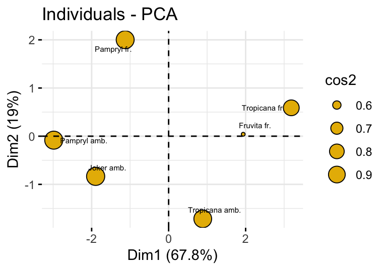
圖 81.7: Score plot/individual plot of the orange data.
細心觀察的話,你會發現圖 81.7 中各個橙汁 (個體,individual) 的座標其實是來自於PCA分析結果中第一和第二主成分變量的結果,展示在第一和第二主成分變量構成的平面。該平面解釋了總體數據慣性 (inertia) 的 86.82% (= 67.77% + 19.05%)。其中第一個主成分 Dim.1 把 Tropicana fr. 和 Pampryl amb. 兩種橙汁分別歸類在最右邊和最左邊。這是因爲原始數據中 Tropicana fr. 是 Odour.typicality 得分最高 Bitternes 得分倒數第二低,同時 Pampryl amb. 則是在這兩個項目上得分分別是最低和最高。也就是說這兩種橙汁在這兩個項目上得分分別是左右兩種極端,所以首先在第一主成分中把這兩中橙汁分離開來。接下來,第二主成分變量 Dim.2 則是將第一主成分成功分離開的兩個個體(橙汁)從數據中拿掉以後,剩下的四種橙汁的分類。可以看到第二個主成分軸,把 Pampryl fr. 和 Tropicana amb. 兩種橙汁放在了該軸的兩個極端,這是因爲 Pampryl fr. 在 Intensity.of.taste 項目上得分最高,而 Tropicana amb. 在拿掉了第一主成分分離的兩種橙汁之後,在 Odour.intensity 項目上得分最低。
回到 R 幫忙分析的主成分結果報告來:
##
## Call:
## PCA(X = orange[, 1:7], ncp = 7, graph = FALSE)
##
##
## Eigenvalues
##                        Dim.1   Dim.2   Dim.3   Dim.4   Dim.5
## Variance               4.744   1.333   0.820   0.084   0.019
## % of var.             67.767  19.047  11.712   1.200   0.274
## Cumulative % of var.  67.767  86.814  98.526  99.726 100.000
##
## Individuals
##                        Dist    Dim.1    ctr   cos2    Dim.2    ctr   cos2    Dim.3    ctr   cos2
## Pampryl amb.       |  3.029 | -2.984 31.288  0.970 | -0.082  0.085  0.001 | -0.333  2.254  0.012 |
## Tropicana amb.     |  1.976 |  0.886  2.761  0.201 | -1.715 36.771  0.753 | -0.087  0.154  0.002 |
## Fruvita fr.        |  2.595 |  1.937 13.182  0.557 |  0.040  0.020  0.000 |  1.710 59.450  0.434 |
## Joker amb.         |  2.094 | -1.896 12.631  0.820 | -0.834  8.686  0.158 | -0.154  0.481  0.005 |
## Tropicana fr.      |  3.512 |  3.186 35.660  0.823 |  0.589  4.335  0.028 | -1.345 36.774  0.147 |
## Pampryl fr.        |  2.338 | -1.129  4.479  0.233 |  2.002 50.102  0.733 |  0.209  0.887  0.008 |
##
## Variables
##                       Dim.1    ctr   cos2    Dim.2    ctr   cos2    Dim.3    ctr   cos2
## Odour.intensity    |  0.460  4.452  0.211 |  0.754 42.694  0.569 | -0.468 26.771  0.219 |
## Odour.typicality   |  0.985 20.468  0.971 |  0.134  1.350  0.018 | -0.058  0.417  0.003 |
## Pulpiness          |  0.722 10.977  0.521 |  0.617 28.519  0.380 |  0.298 10.826  0.089 |
## Intensity.of.taste | -0.650  8.902  0.422 |  0.429 13.797  0.184 |  0.626 47.747  0.391 |
## Acidity            | -0.913 17.561  0.833 |  0.348  9.100  0.121 | -0.021  0.056  0.000 |
## Bitterness         | -0.935 18.420  0.874 |  0.188  2.651  0.035 | -0.285  9.936  0.081 |
## Sweetness          |  0.955 19.220  0.912 | -0.159  1.889  0.025 |  0.187  4.246  0.035 |
可以看到第一部分是特徵值(eigenvalue)的結果描述,第二部分是個人 (individual) 的分析報告:
...{omitted}...
Individuals
                       Dist    Dim.1    ctr   cos2    Dim.2    ctr   cos2
Pampryl amb.       |  3.029 | -2.984 31.288  0.970 | -0.082  0.085  0.001
Tropicana amb.     |  1.976 |  0.886  2.761  0.201 | -1.715 36.771  0.753
Fruvita fr.        |  2.595 |  1.937 13.182  0.557 |  0.040  0.020  0.000
Joker amb.         |  2.094 | -1.896 12.631  0.820 | -0.834  8.686  0.158
Tropicana fr.      |  3.512 |  3.186 35.660  0.823 |  0.589  4.335  0.028
Pampryl fr.        |  2.338 | -1.129  4.479  0.233 |  2.002 50.102  0.733
...{omitted}...
其中,
Dist是每個個體(行數據),到座標軸原點 (平均重心位置) 的距離。此數據中距離原點最遠的兩種橙汁是Pampryl amb.(最左邊) 和Tropicana fr.(最右邊)。Dim.1是該個體,在第一個主成分變量座標軸上的座標。ctr是該個體在第一個主成分變量提取時貢獻的百分比。cos2是該個體在該主成分變量上投影的慣性除以該個體本身的慣性所佔的比例,又叫做該個體對相應主成分變量的代表性評價 (the quality of representation of an individual \(i\) on the principle component \(s\) is measured by the distance between the point within the space \(u_s\) and the projection on the component)。
\[ \text{quality of representation}_s(i) = \frac{\text{Projected inertia of }i \text{ on } u_s}{\text{Total inertia of }i} = \cos^2\theta_i^s \]
PCA報告的下半部分,是關於數據中變量與變量之間關係的分析結果。
Variables
                      Dim.1    ctr   cos2    Dim.2    ctr   cos2    Dim.3    ctr   cos2
Odour.intensity    |  0.460  4.452  0.211 |  0.754 42.694  0.569 | -0.468 26.771  0.219 |
Odour.typicality   |  0.985 20.468  0.971 |  0.134  1.350  0.018 | -0.058  0.417  0.003 |
Pulpiness          |  0.722 10.977  0.521 |  0.617 28.519  0.380 |  0.298 10.826  0.089 |
Intensity.of.taste | -0.650  8.902  0.422 |  0.429 13.797  0.184 |  0.626 47.747  0.391 |
Acidity            | -0.913 17.561  0.833 |  0.348  9.100  0.121 | -0.021  0.056  0.000 |
Bitterness         | -0.935 18.420  0.874 |  0.188  2.651  0.035 | -0.285  9.936  0.081 |
Sweetness          |  0.955 19.220  0.912 | -0.159  1.889  0.025 |  0.187  4.246  0.035 |
根據這個結果繪製的變量相關關係圖如下:
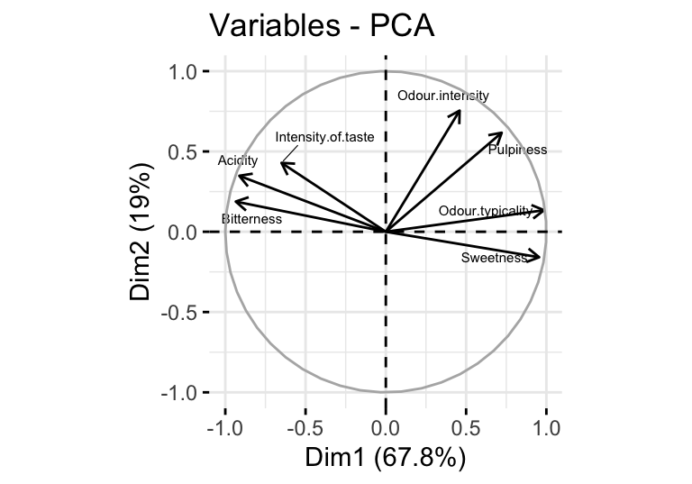
圖 81.8: Variable plot of the orange data.
- 在第一個主成分軸上 (
Dim.1),正相關的變量Odour.intensity, Odour.typicality, Pulpiness, Sweetness被歸類在右半球,而負相關的變量Intensity.of.taste, Acidity, Bitterness則被歸類在第一主成分軸的左半球。 - 相似地,在第二個主成分軸上 (
Dim.2),只有負相關的Sweetness被歸類在下半球。 - 每個變量從原點出發時的箭頭長度越長
cos2,代表它在該主成分軸上代表質量更好 (the quality of representation of the variable on the component)
如果你願意,且數據和變量不至於多到眼花繚亂,我們還可以把個體圖和變量圖結合起來觀察:
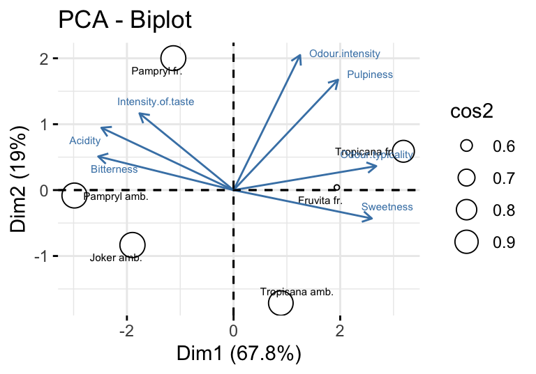
圖 81.9: Biplot of the orange data.
81.5 在PCA圖形中加入補充變量和補充個體 (supplementary elements)
在橙汁數據中,除了有美食家給出的各個味道項目的評分之外,其實還有各個橙汁的物理化學特性數據。
| Glucose | Fructose | Saccharose | Sweetening.power | pH | Citric.acid | Vitamin.C | Way.of.preserving | Origin | |
|---|---|---|---|---|---|---|---|---|---|
| Pampryl amb. | 25.32 | 27.36 | 36.45 | 89.95 | 3.59 | 0.84 | 43.44 | Ambient | Other |
| Tropicana amb. | 17.33 | 20.00 | 44.15 | 82.55 | 3.89 | 0.67 | 32.70 | Ambient | Florida |
| Fruvita fr. | 23.65 | 25.65 | 52.12 | 102.22 | 3.85 | 0.69 | 37.00 | Fresh | Florida |
| Joker amb. | 32.42 | 34.54 | 22.92 | 90.71 | 3.60 | 0.95 | 36.60 | Ambient | Other |
| Tropicana fr. | 22.70 | 25.32 | 45.80 | 94.87 | 3.82 | 0.71 | 39.50 | Fresh | Florida |
| Pampryl fr. | 27.16 | 29.48 | 38.94 | 96.51 | 3.68 | 0.74 | 27.00 | Fresh | Other |
我們可以把這些沒有用於計算主成分分析的變量 (active variables),和其餘的輔助性變量 (supplementary variables) 同時繪製在變量相關係數圓盤圖中。此時我們只需要在進行PCA運算的時候告訴R這些變量是輔助性的連續/分類變量即可:
## $coord
##                         Dim.1       Dim.2         Dim.3        Dim.4       Dim.5
## Glucose          -0.572454497  0.31123036  0.0263849025 -0.208332016 -0.72892600
## Fructose         -0.561054870  0.31451133 -0.0084203081 -0.181973281 -0.74371694
## Saccharose        0.750440168  0.14492075  0.3246761207 -0.075192796  0.55205886
## Sweetening.power  0.300767457  0.67471255  0.4895557731 -0.389880490 -0.25026037
## pH                0.879663611 -0.23629707  0.1935892274  0.245926101  0.26907097
## Citric.acid      -0.739370266 -0.12160048 -0.1957416737 -0.278669842 -0.56795532
## Vitamin.C        -0.044575912 -0.31698263 -0.2545161911 -0.905066399  0.11666756
##
## $cor
##                         Dim.1       Dim.2         Dim.3        Dim.4       Dim.5
## Glucose          -0.572454497  0.31123036  0.0263849025 -0.208332016 -0.72892600
## Fructose         -0.561054870  0.31451133 -0.0084203081 -0.181973281 -0.74371694
## Saccharose        0.750440168  0.14492075  0.3246761207 -0.075192796  0.55205886
## Sweetening.power  0.300767457  0.67471255  0.4895557731 -0.389880490 -0.25026037
## pH                0.879663611 -0.23629707  0.1935892274  0.245926101  0.26907097
## Citric.acid      -0.739370266 -0.12160048 -0.1957416737 -0.278669842 -0.56795532
## Vitamin.C        -0.044575912 -0.31698263 -0.2545161911 -0.905066399  0.11666756
##
## $cos2
##                         Dim.1       Dim.2          Dim.3        Dim.4       Dim.5
## Glucose          0.3277041510 0.096864337 0.000696163079 0.0434022288 0.531333120
## Fructose         0.3147825674 0.098917374 0.000070901589 0.0331142749 0.553114882
## Saccharose       0.5631604458 0.021002025 0.105414583332 0.0056539566 0.304768989
## Sweetening.power 0.0904610632 0.455237031 0.239664854983 0.1520067964 0.062630255
## pH               0.7738080690 0.055836307 0.037476788962 0.0604796473 0.072399188
## Citric.acid      0.5466683910 0.014786677 0.038314802810 0.0776568810 0.322573248
## Vitamin.C        0.0019870119 0.100477991 0.064778491512 0.8191451868 0.013611319
然後用下面的代碼繪製包含了輔助性變量的變量相關圓盤圖:
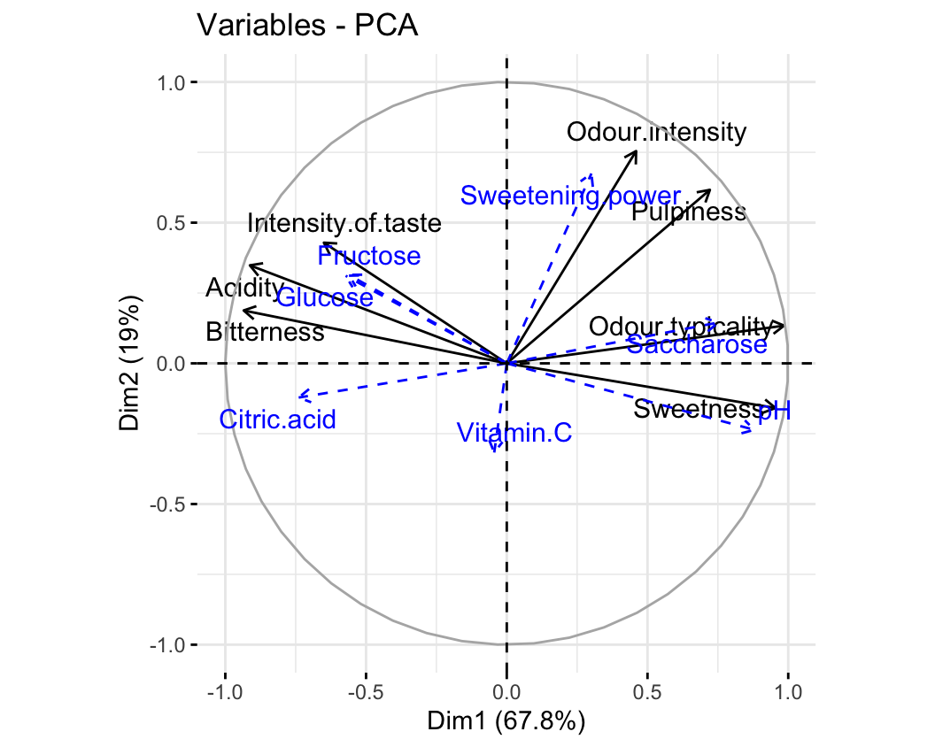
圖 81.10: Orange juice data: representation of the active and supplementary variables (in blue).
如圖 81.10 所示,第一個主成分變量分離的左右半球的橙汁味道特徵,和他們的物理特性其實是相呼應的。例如,pH 值出現在了圓盤的右半邊,靠近 Sweetness 這一變量。因爲 pH 越高,酸度越低,那麼味道也就越甜,這是合理的。另外一個有趣的現象是,蔗糖 saccharose 含量高的橙汁,pH 越高,味道越甜。在圓盤的左邊,是蔗糖在酸環境下分解之後產生的果糖和葡萄糖,所以果糖葡萄糖反而和酸度 Acidity 相關性高,因爲橙汁中果糖葡萄糖含量高意味着蔗糖被酸分解。
由此可見,PCA是一個對數據進行初步描述和探索時十分有力的工具。所以,在回歸模型選擇變量之前,建議可以對數據先進行主成分分析,並且把預備考慮放在回歸模型的解釋變量部分的變量用於PCA主成分分析,把想要做預測的變量作爲輔助性變量投射到主成分分析的變量相關圖中,觀察解釋變量之間可能存在的相關性,有助於選取合適的解釋變量。
81.5.1 展示分類輔助性變量和個體的關係
根據不同的儲存方式,兩類的橙汁區別很清楚。
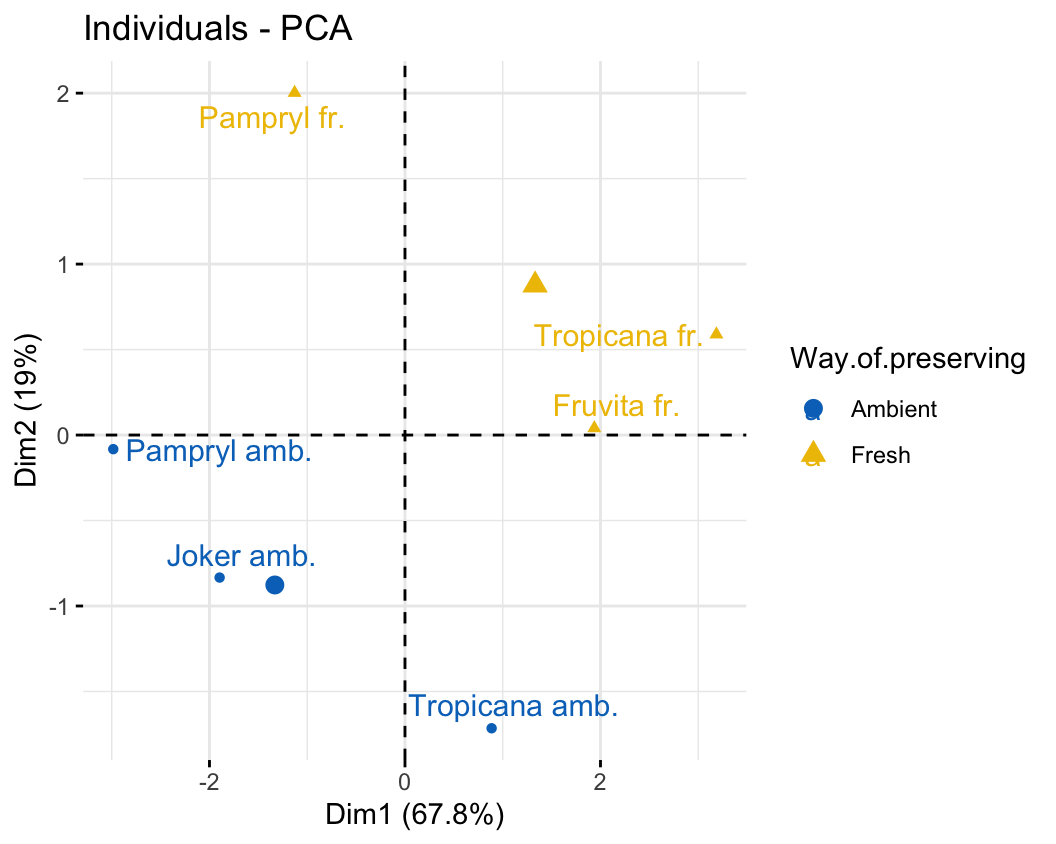
圖 81.11: Plane representation of the scatterplot of individuals with a supplementary categorical variable (way of preserving).
根據橙子的產地區分繪製的個人圖:
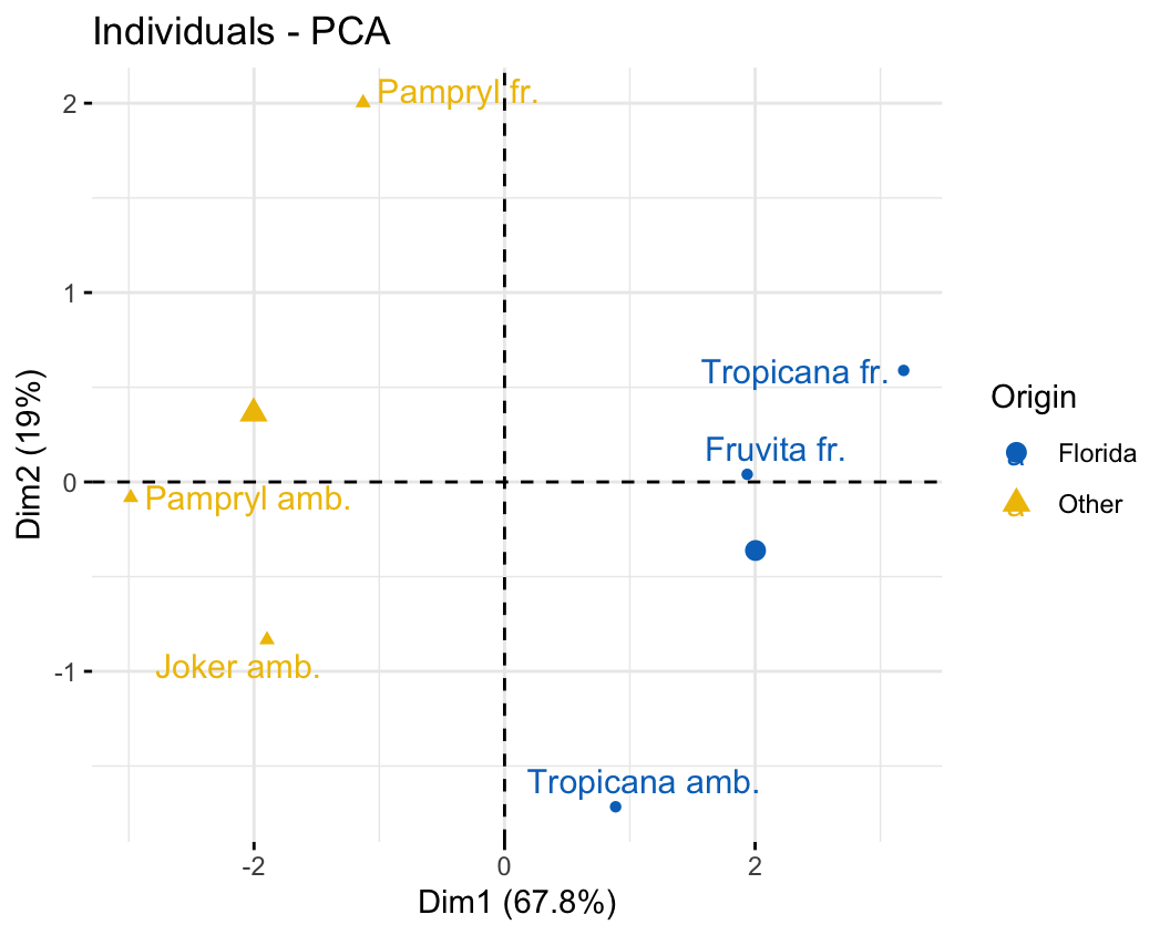
圖 81.12: Plane representation of the scatterplot of individuals with a supplementary categorical variable (origin).
81.6 Cluster analysis/PCA practical
本次練習完成時,你將學會:
- 如何使用聚類分析,和主成分分析法來探索一組多變量數據之間的關係;
- 理解並懂得如何選取合適的距離測量尺度,和聚類分析方法;
- 繪製並能夠解釋由多層聚類分析算法 (hierarchical clustering algorithm) 獲得的樹狀圖;
- 使用主成分分析法對數據進行座標轉換,計算多個變量之間的方差,協方差矩陣,懂得如何判斷保留主成分的個數;
- 通過把數據繪製在較低維度的主成分座標軸上來判斷數據中可能存在的潛在分層/分組。
81.6.1 使用的數據和簡單背景知識
假設你是一名生物測量技術公司的統計師,現在有這樣一組數據,包含了對某植物測量的4種生物標幟物(biomarkers)。據報道,這四種成分或許能減少你公司生產的某藥物引起的副作用。爲了嘗試分析該植物的生物特性,從該植物的50個不同樣本中,測量了這4種生物標幟物的濃度。你的任務之一是對數據進行初步分析,彙報任何你找到的可能存在的顯著特徵差異。
- 在R裏讀入你的數據,看看這4種生物標幟物的簡單統計量和分佈,它們用的是相同的測量單位嗎?
## # A tibble: 6 × 4
##       bm1     bm2     bm3     bm4
##     <dbl>   <dbl>   <dbl>   <dbl>
## 1  17.4    78.6   101.    109.
## 2  87      30.1    79.1     6.60
## 3   0.100   0.600   0.900   0.200
## 4 106      10      44.6    57.6
## 5 141.    122     115.    123.
## 6 0.5 0.800 0.200 0.5##
## No. of observations = 50
##
## Var. name obs. mean median s.d. min. max.
## 1 bm1 50 56.6 47.55 48.05 0 143
## 2 bm2 50 53.21 52.7 45.13 0 143.6
## 3 bm3 50 61.43 55.25 51.47 0.2 147.9
## 4 bm4 50 57.43 56.75 45.45 0.1 146.1## vars n mean sd median trimmed mad min max range skew kurtosis se
## bm1 1 50 56.60 48.05 47.55 53.36 66.05 0.0 143.0 143.0 0.27 -1.38 6.80
## bm2 2 50 53.21 45.13 52.70 49.62 59.45 0.0 143.6 143.6 0.43 -1.07 6.38
## bm3 3 50 61.43 51.47 55.25 58.86 69.76 0.2 147.9 147.7 0.27 -1.47 7.28
## bm4 4 50 57.43 45.45 56.75 54.71 52.41 0.1 146.1 146.0 0.32 -1.12 6.43觀察這四個生物標幟物的簡單統計量,似乎可以認爲它們使用的應該是相似或者相同的測量單位。它們的均值在53至61之間,標準差分佈在45-51之間,而且最大值最小值之間的範圍也十分接近。
- 這些生物標幟物能否單獨提供關於該植物的某部分特徵信息呢?思考我們該如何回答這個問題(提示:計算這些指標直接的相關係數)
我們可以通過計算這四個生物標幟物濃度測量值之間的相關係數,來觀察它們之間是否具有相似性或者是否提供了部分相似的信息。
##            bm1        bm2        bm3        bm4
## bm1 1.00000000 0.49826220 0.59414820 0.26769269
## bm2 0.49826220 1.00000000 0.50574946 0.33347350
## bm3 0.59414820 0.50574946 1.00000000 0.32094816
## bm4 0.26769269 0.33347350 0.32094816 1.00000000
從相關係數矩陣的計算結果來看,平均地,這四個生物標幟物濃度之間具有一定程度的相關性。其中,生物標幟物1和3之間呈現了四者之間最高的樣本相關係數 \((r_{13} = 0.5941)\),生物標幟物1和4之間的相關係數則最小 \((r_{14} = 0.2677)\)。
- 請描述前一步中我們計算的相關係數矩陣的維度(dimension)。
該相關係數矩陣的維度是 \(4\times4\),事實上,這個矩陣的維度是由我們想要觀察分析的樣本中測量變量的個數決定的(在這裏就是四個生物標幟物)。但是這個相關係數的矩陣並不適合用於做聚類分析 (cluster analysis),因爲相關係數本身反映的是變量之間的關係 (between variables),並非觀察對象 (between subjects) 之間的距離(即,不是我們關心的用來把50個樣本進行分組歸類的距離變量)。
- 再次思考問題1.的答案,思考並選擇合適的測量不同樣本個體之間距離 (distance) 的度量衡。嘗試使用簡單的聚類分析命令對樣本進行分類。
由於每個生物標記物在所有樣本中的數值基本在相似的比例或者刻度,每個標幟物在這個樣本中的標準差/方差數值也較爲相近。我們嘗試用連續變量最常見的均值測量距離指標:
# prepare hierarchical cluster
hc <-  hclust(dist(plant), "ave")


plot(hc, cex = 0.8, hang = -1,
     main = "", ylab = "L2 dissimilarity measure",
     xlab = "No. of specimen")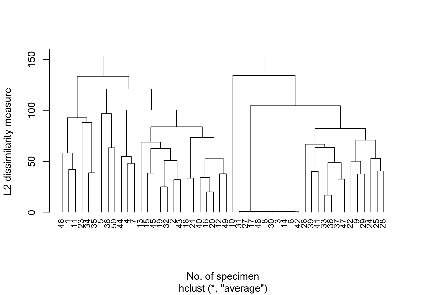
圖 81.13: Dendrogram for L2_avlink cluster analysis
可以觀察到,樣本編號 31, 27, 17, 48, 8, 30, 3, 14, 6, 42 很快就聚合成爲一組。且這些樣本和其他樣本被聚類在不同組的過程一直維持到差異性達到100以上。我們還可以注意到,聚類過程中其他的分支呈現相對對稱的形狀。
- 從簡單的歐幾里得距離改成歐幾里得距離平方來測量樣本之間的距離的話,圖形會變成什麼樣?
hc <- hclust(dist(plant)^2)

plot(hc, cex = 0.8, hang = -1,
     main = "", ylab = "L2squared dissimilarity measure",
     xlab = "No. of specimen", sub = "")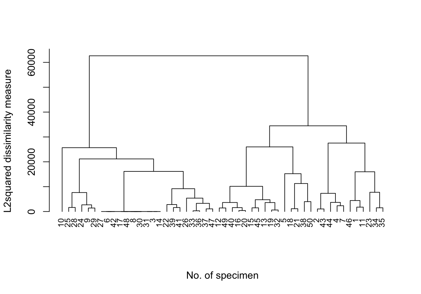
圖 81.14: Dendrogram for L2sq_avlink cluster analysis
當使用歐幾里得距離的平方作爲樣本間隔的度量衡時,我們發現聚類的過程其實總體來說和使用歐幾里得距離本身並無本質上的區別。只是在差異性較低的地方聚類加速 (squeeze the dissimilarities at the lower end),並且在較大的聚類區分之間變得更加明顯,視覺效果上更容易區分。
如果說,不用歐幾里得平方,而是使用簡單的曼哈頓距離 (L1 度量衡),那麼圖形則又會呈現爲:
plot(cluster::agnes(plant, metric = "manhattan", stand = F), which.plots = 2, hang = -1,
     xlab = "No. of specimen", main = "", ylab = "L1 dissimilarity measure", sub = "", cex = 0.8)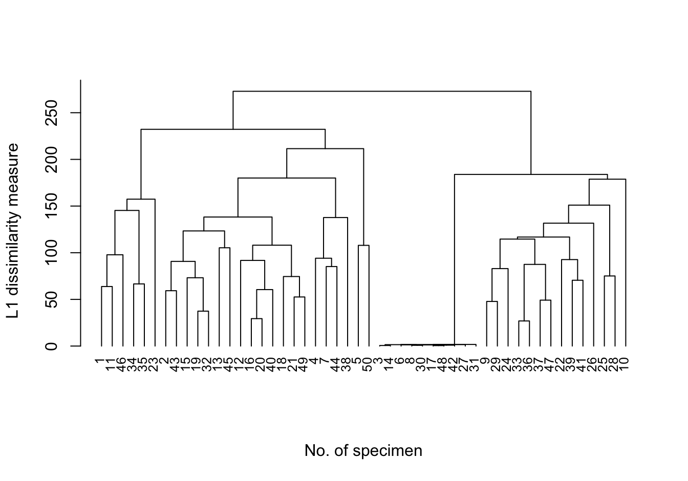
圖 81.15: Dendrogram for L1_avlink cluster analysis
可以看出,當使用曼哈頓距離做度量衡時,聚類的過程和之前的沒有本質上的區別,但是圖形的樹狀分支上似乎不再左右對稱。
- 接下來使用歐幾里得距離做度量衡,與上面的嘗試不同,這裏我們嘗試用完全連接,和單連接