第 86 章 非參數法分析生存數據
86.1 本章概要
本章內容包括
- 使用非參數方法(分別是Kaplan-Meier法,和生命表法)估計生存方程,累計風險度方程,同時考慮刪失值。
- 使用 Greenwood 表達式 (Greenwood’s) 計算非參數法獲得的參數估計的不確定性(即信賴區間)。
- 製作生存分析非參數法的繪圖。
- 非參數法比較不同組間(治療組對照組)的生存時間。
- 學會並理解如何實施 log rank test 比較兩組之間生存時間模式的不同 (pattern of survival times)
- 在R中實際操作非參數法分析生存數據,並理解其輸出結果的含義。
86.2 生存分析中的非參數分析法
非參數法分析生存數據其實是所有人在分析生存數據時應該着手做的第一件事。
- 非參數法可以對生存時間不必進行任何參數分布 (parametric assumption) 的假設,初步地估計生存方程和累積風險度方程;
- 使用非參數法可以用生存曲線圖的方式直觀地展示生存數據,包括刪失值在數據中的存在也可以通過圖表來表現出來;
- 非參數法可以初步地對不同組/羣之間生存曲線的變化進行比較;
- 通過非參數法對生存數據進行初步分析之後,可以對其後更加複雜的生存數據建模過程提供有參考價值的背景信息。
86.3 Kaplan-Meier 法分析生存方程
86.3.1 當數據中沒有刪失值
如果,研究對象裏的每個人都發生了事件,那麼研究對象裏的每個人身上都觀察到了生存時間,自然而然地特定時間 \(t\) 時的生存方程是:
\[ \hat{S}(t) = \frac{\text{number of individuals with survival time} > t}{\text{total number of individuals}} \]
在每個觀察到事件的時間點 \(t_1 < t_2 < t_3 < \cdots < t_K\),我們可以計算該時間點的生存方程,然後假定兩個事件的時間點之間的生存概率保持不變,就可以繪制出一個階梯形狀的生存曲線。也就是說,只有在觀察到事件的那些時間點上,生存方程得到定義。
Example 86.1 依舊是白血病患者數據,估計對照組的生存方程。在這個白血病患者數據中,對照組中並沒有刪失值,正好可以用來展示沒有刪失值時,生存方程的計算過程。對照組中有21名白血病患者,我們感興趣的事件是癌症是否緩解,此時的生存時間是,緩解前的時間(單位週)他們的數據被總結在下面的表格中,其中治療組的時間後面某些患者的星號 (*) 表示這些患者無緩解,是刪失值:
| Control group | 1,1,2,2,3,4,4,5,5,8,8,8,8,11,11,12,12,15,17,22,23 |
|---|---|
| Treatment group | 6*,6,6,6,7,9*,10*,10,11*,13,16,17*,19*,20*,22,23,25*,32*,32*,34*,35* |
對照組中患者的實際觀測數據計算獲得的生存方程總結在下面的表格中:
| \(t_j\) | Number of events \(d_j\) | \(\hat{S}(t_j)\) |
|---|---|---|
| 1 | 2 | 19/21 = 0.90 |
| 2 | 2 | 17/21 = 0.81 |
| 3 | 1 | 16/21 = 0.76 |
| 4 | 2 | 14/21 = 0.67 |
| 5 | 2 | 12/21 = 0.57 |
| 8 | 4 | 8/21 = 0.38 |
| 11 | 2 | 6/21 = 0.29 |
| 12 | 2 | 4/21 = 0.19 |
| 15 | 1 | 3/21 = 0.14 |
| 17 | 1 | 2/21 = 0.10 |
| 22 | 1 | 1/21 = 0.05 |
| 23 | 1 | 0 |
上面表格中估計的生存方程可以用下圖 86.1 來表示。可見這樣的生存方程繪製成的生存曲線其實是呈現階梯狀的。這也是爲什麼我們說在這樣的非參數過程中,生存方程在觀察到事件的兩個時間點之間默認生存方程是恆定不變的。
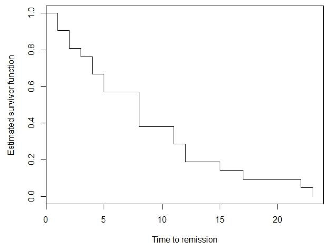
圖 86.1: Estimated survivor function corresponding to the leukaemia data in the control group.
86.3.2 當數據中有刪失值
前一小節提到的非參數法繪制生存時間曲線的方法,其實完全可以拓展到含有刪失值的生存數據中。同樣地,用 \(t_1 < t_2 < t_3 < \cdots < t_K\) 表示發生事件的觀察對象的生存時間。我們可以用以下的步驟來拓展生存時間曲線的繪制思路:
- 首先定義 \(h_j\) 作爲時間 \(t_j\) 時期的風險率 (hazard rate),那麼每個發生事件的對象的風險和生存時間就有了各自的關聯 \(h_1, h_2, \cdots, h_k\);
- 在時間點 \(t_1\) 時,隊列中的全部對象中,沒有發生事件的概率是 \(1-h_1\);
- 在時間點 \(t_2\) 時,隊列中的全部對象中,在時間 \(t_1, t_2\) 時都沒有發生事件的概率是 \((1-h_1)(1-h_2)\);
- 所以,生存方程就是,任何一個人,在任何一個時間點,在隊列中,且不發生事件的概率 \[S(t_j) = \prod_{k=1}^j(1-h_k)\]
此時,每個時間點風險度方程的無偏估計爲,該時間點中在隊列中發生事件的人數 \(d_j\) 除以當時在隊列中的人數 \(n_j\):
\[ \hat h_j = \frac{d_j}{n_j} \]
用上面的這些初步結果,可以推導出在時間點 \(t_j\) 時,隊列中的生存方程是:
\[ \hat S(t_j) = \prod_{k=1}^j (1-\hat h_k) = \prod_{k=1}^j ( 1- \frac{d_k}{n_k}) \]
它的更加一般化形式就是我們常常念叨的那個生存方程的 Kaplan-Meier 估計量,它的別名是 “the product limit estimate”:
\[ \begin{equation} \hat S(t) = \prod_{j|t_j \leqslant t} (1 - \frac{d_j}{n_j}) \end{equation} \tag{86.1} \]
Example 86.2 下表羅列了某個白血病患者治療組生存數據的 Kaplan-Meier 生存方程估計和他們的計算過程,其中值得注意的是,如果生存表格中某時間點 (年或月或日,取決於你的研究使用的時間刻度) 同時有事件 (event) 和刪失 (censoring),習慣上是默認刪失發生在事件發生之前:
| Survival time \((t_j)\) and censoring time | Number at risk | Number of events | Number of censorings | \(\hat{S}(t_j)\) |
|---|---|---|---|---|
| 6 | 21 | 3 | 1 | (1-3/21) = 0.857 |
| 7 | 17 | 1 | 0 | (1-3/21)(1-1/17) = 0.807 |
| 9 | 16 | 0 | 1 | – |
| 10 | 15 | 1 | 1 | (1-3/21)(1-1/17)(1-1/15) = 0.753 |
| 11 | 13 | 0 | 1 | – |
| 13 | 12 | 1 | 0 | 0.69 |
| 16 | 11 | 1 | 0 | 0.627 |
| 17 | 10 | 0 | 1 | – |
| 19 | 9 | 0 | 1 | – |
| 20 | 8 | 0 | 1 | – |
| 22 | 7 | 1 | 0 | 0.538 |
| 23 | 6 | 1 | 0 | 0.448 |
| 25 | 5 | 0 | 1 | – |
| 32 | 4 | 0 | 2 | – |
| 34 | 2 | 0 | 1 | – |
| 35 | 1 | 0 | 1 | – |
下圖 86.2 則繪製了治療組處理了刪失值後的生存方程數據。
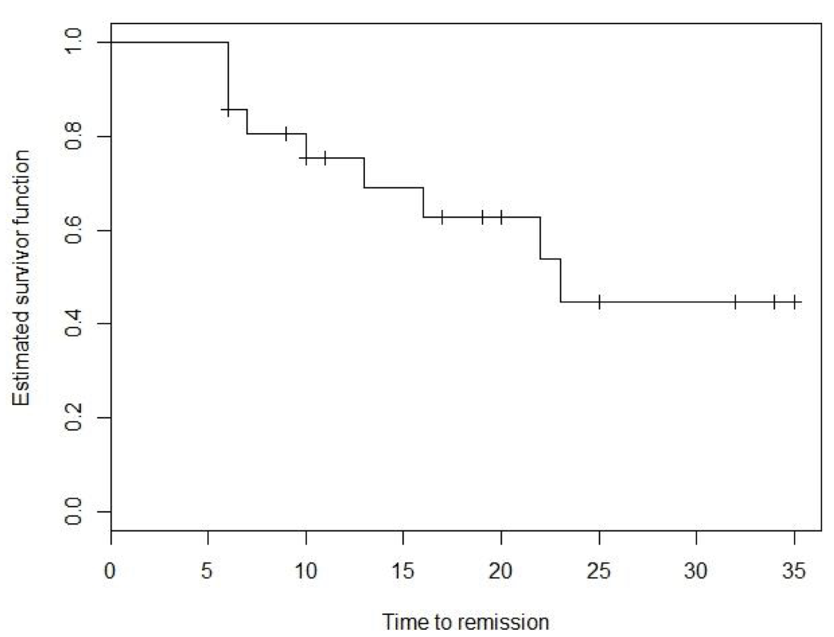
圖 86.2: Kaplan-Meier survival curve for leukaemia patients in the treatment group.
86.4 Kaplan-Meier 數據的信賴區間的估計
Greenwood’s 公式的推導:
如何推導獲得生存估計 \(\hat{S}(t_j)\) 的方差呢?
利用方程 (86.1) 的對數:
\[ \begin{aligned} \text{Var}\{ \text{log}\hat{S}(t) \} & = \text{Var}\{ \text{log}\prod_{j|t_j \leqslant t} (1 - \hat{h}_j)\} \\ & = \text{Var}\{ \sum_{j|t_j \leqslant t} \text{log}(1-\hat{h}_j)\} \\ & = \sum_{j|t_j \leqslant t}\text{Var}\{ \text{log}(1-\hat{h}_j) \} \end{aligned} \]
接下來利用線性近似原則 (linear approximation),也就是英国数学家泰勒的一次近似泰勒展开法 (first order Taylor series approximation):
\[ \begin{equation} \text{log} (1-\hat{h}_j) \approx \text{log}(1-h_j) + (\hat{h}_j - h_j)/(1-h_j) \end{equation} \tag{86.2} \]
這個近似公式可以讓我們得到其方差爲:
\[ \text{Var}\{ \text{log}(1-\hat{h}_j) \} \approx \frac{\text{Var}(\hat{h}_j)}{(1-h_j)^2} \]
这个就是大名鼎鼎的 Delta 法。
接下來需要推導風險 (hazard) \(\hat{h}_j\) 的方差,注意,在時間 \(t_j\) 時, 事件發生次數 \(d_j\) 其實是服從如下的二項分布:
\[ d_j \sim \text{Binomial}(n_j, h_j) \]
所以,
\[ \text{Var}(\hat{h}_j) = \frac{\text{Var}(d_j)}{n_j^2} \]
根據伯努利分布 (Chapter 4) 和二項分布 (Chapter 5) 的性質:
\[ \text{Var}(\hat{h}_j) = \frac{\text{Var}(d_j)}{n_j^2} = \frac{n_jh_j(1-h_j)}{n_j^2} = \frac{h_j(1-h_j)}{n_j} \]
綜上可得:
\[ \text{Var}\{ \text{log}(\hat{S}(t)) \} = \sum_{j|t_j \leqslant t}\frac{h_j}{n_j(1-h_j)} \]
這裏再對 \(\log(\hat{S}(t))\) 用一次線性近似:
\[ \log\hat{S}(t) \approx \log S(t) + \frac{\hat{S}(t) - S(t)}{S(t)} \]
所以其實
\[ \text{Var}\{ \log (\hat{S}(t)) \} = \frac{\text{Var}\{ \hat{S}(t) \}}{S(t)^2} \]
最終我們獲得 Greenwood’s 公式:
\[ \begin{equation} \text{Var}\{ \hat{S}(t) \} = \hat{S}(t)^2\sum_{j|t_j \leqslant t}\frac{h_j}{n_j(1-h_j)} \end{equation} \tag{86.3} \]
獲得生存方程的方差以後,接下來就是 95% 信賴區間的推導:
\[ \hat{S}(t) \pm 1.96 \sqrt{\text{Var}\{ \hat{S}(t) \}} \]
這裏獲得的 Kaplan-Meier 信賴區間是沒有錯的,但是在某些較爲極端的生存數據中 (時間接近 0, 或者時間接近追蹤結束),這個公式可能導致計算獲得的信賴區間超過 \((0,1)\)。因爲這裏我們假定的是生存概率近似服從正態分布時,才能使用的信賴區間公式。另一個改良版本的區間公式可以避免出現不正常的信賴區間。它需要對生存數據進行數學轉換。常用的生存數據的數學轉換是 \(\log\{-\log \hat{S}(t) \}\)。利用上面推導 Greenwood’s 公式 (86.3) 時相似的過程,我們可以獲得該轉換過後的方差是:
\[ \begin{equation} \text{Var}\{ \log\{-\log \hat{S}(t)\} \} \approx \frac{\text{Var}\{\log\hat{S}(t) \}}{\{ \log S(t) \}^2} \end{equation} \tag{86.4} \]
如果使用 \(v^2(t)\) 來標記上式 (86.4) 時,有
\[ \begin{aligned} \log\{- \log \hat{S}(t) \} - 1.96v(t) & < \log\{-\log S(t) \} < \log\{- \log \hat{S}(t) \} + 1.96v(t) \\ \text{Taking the exponential:} & \\ \{ -\log \hat{S}(t) \} \exp(-1.96v(t)) & < -\log S(t) < \{ -\log \hat{S}(t) \} \exp(1.96v(t)) \\ \text{Multiply everything by } & -1: \\ \{ \log \hat{S}(t) \} \exp(1.96v(t)) & < \log S(t) < \{ \log \hat{S}(t) \} \exp(-1.96v(t)) \\ \text{Take the exponential again:} & \\ \hat{S}(t)^{\exp(1.96v(t))} & < S(t) < \hat{S}(t)^{\exp(-1.96v(t))} \end{aligned} \]
所以,這個校正版本的生存方程信賴區間公式就是:
\[\hat{S}(t)^{\exp\{ \mp1.96 v(t)\}}\]
實際上在操作統計軟件的時候你並不需要特別精通上面的推導過程,但是要記得估計非參數法生存方程的 Kaplan-Meier 曲線時,它的95%信賴區間有兩種計算方式,如下圖 86.3 中我們給白血病患者數據中的治療組患者的生存曲線增加了95%信賴區間。
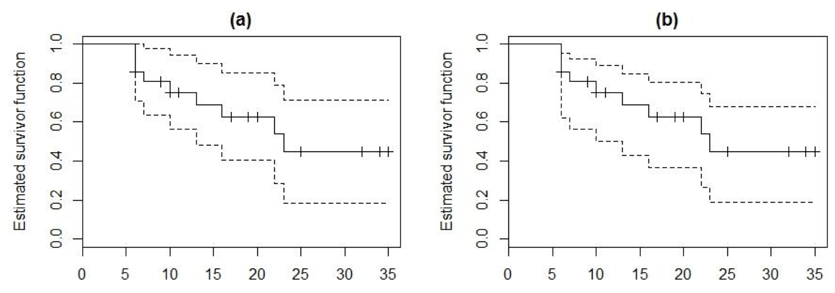
圖 86.3: Kaplan-Meier survival curve (solid line) and 95-percent confidence limits (dotted lines) for leukaemia patients in the treatment group. (a) using Greenwoods formula, (b) using the alternative confidence limits.
86.5 另一種非參數法分析 – 生命表格估計
Kaplan-Meier 估計的生存方程過程中,我們假定的是觀察到事件的時間點是間斷不連續的,也就是哪個事件發生在哪個時間點,是可以被精確觀察到的。然而,現實比較骨感的時候,你的數據可能只有生命表格,也就是常見的如一年內本市死亡人口多少多少人這樣,事件發生在某個時間區間內的類型數據。因爲此時無法特定每個死亡人口發生死亡時的確切時間日期。此時可以利用生命表格計算。
我們假定,某個隨訪時間可以被分爲許許多多的時間區間 \(I_1, I_2, \cdots, I_K\),且這些時間區間並不一定需要等間距。另外,用 \(d_j\) 表示在時間區間 \(I_j\) 中發生的事件次數,在該時間段的起始點的時刻,有 \(n_j\) 個觀察對象 (number of individuals at risk at the start of interval \(I_j\)),其中在下一段時間開始之前,有 \(m_j\) 個刪失值。用這些數學標記來表示時間段 \(I_j\) 中發生事件的概率 (前提是這 \(n_j\) 個觀察對象在時間段 \(I_j\) 開始前還沒有發生事件):
\[p_j = \frac{d_j}{n_j - m_j/2}\]
分母中使用了 \(m_j/2\) 是由於我們無法確定事件發生和刪失值發生的時間在這個時間段 \(I_j\) 中是如何分布的,所以我們只能假定/默認他們平均的分布在時間段 \(I_j\) 中點的兩側。如此,生命表法計算的生存方程公式就是:
\[ \hat{S}(t) = \prod_{k = 1}^j(1-p_k) \text{ for } t_j \leqslant t < t_{j+1} \]
你可以看出,生命表的推算生存方程,其實和 Kaplan-Meier 法很接近,你同樣可以使用 Greewood’s 的公式 (用 \(n_j - m_j/2\) 替換掉 \(n_j\) 即可) 獲取生命表生存方程的方差用於計算其信賴區間。
Example 86.3 心絞痛患者死亡追蹤: 生命表格的制作例子 (選自 (Belle et al. 2004))。本例子中,2418 名男性心絞痛患者被收入研究中並追蹤其死亡結果,記錄數據中包括患者死亡的日期和患者離開研究的時間。下面的表格是追蹤前十年的數據:
| Year | \(n_j\) | \(d_j\) | \(m_j\) | \(p_j\) | \(1-p_j\) | \(\hat S(t)\) |
|---|---|---|---|---|---|---|
| 0-1 | 2418 | 456 | 0 | 456/2418 = 0.188 | 0.812 | 0.812 |
| 1-2 | 1962 | 226 | 39 | 226/(1962 - 39/2) = 0.116 | 0.884 | 0.718 |
| 2-3 | 1697 | 152 | 22 | 152/(1697 - 22/2) = 0.090 | 0.910 | 0.653 |
| 3-4 | 1523 | 171 | 23 | 171/(1523 - 23/2) = 0.113 | 0.887 | 0.579 |
| 4-5 | 1329 | 135 | 24 | 135/(1329 - 24/2) = 0.103 | 0.897 | 0.519 |
| 5-6 | 1170 | 125 | 107 | 125/(1170 - 107/2) = 0.112 | 0.888 | 0.461 |
| 6-7 | 938 | 83 | 133 | 83/(938 - 133/2) = 0.095 | 0.905 | 0.417 |
| 7-8 | 722 | 74 | 102 | 74/(722 - 102/2) = 0.110 | 0.890 | 0.371 |
| 8-9 | 546 | 51 | 68 | 51/(546 - 68/2) = 0.100 | 0.900 | 0.334 |
| 9-10 | 427 | 42 | 64 | 42/(427 - 64/2) = 0.106 | 0.894 | 0.299 |
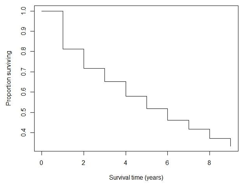
圖 86.4: Men with angina data: Life table estimate of the survivor function.
看圖 86.4 和上面估計的生存概率估計表格,請回答:
- 患者的 5 年以上生存概率是多少? (51.9% 表格第五行)
- 患者的 2.5 年以上生存概率是多少? (71.8% 記住在 2-3 年這段時間內生存概率被假定是不變的)
86.6 兩組之間生存概率的比較
本章目前爲止介紹的非參數法可以用於初步地對生存數據中不同組之間生存概率的比較。我們當然可以給不同組的患者/研究對象估計各自的生存曲線 (和信賴區間) 繪圖比較。
Example 86.4 治療組和對照組白血病患者的生存曲線比較: (本例中,時間是從發病到症狀緩解的時間,所以時間越短,說明療法越好) 下圖繪制的是治療組21名患者和對照組21名患者的生存概率曲線和它們各自的信賴區間。治療組的症狀緩解時間明顯比對照組要長,暗示治療方案可能對患者有不太好的影響。且途中的兩條生存曲線的95%信賴區間也基本沒有重疊。
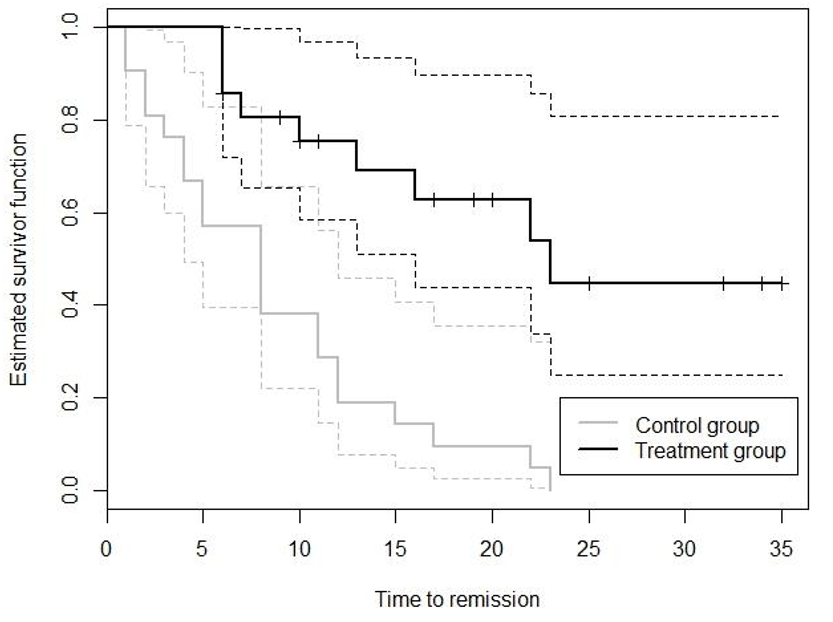
圖 86.5: Kaplain-Meier time-to-remission survival curves (solid lines) in leukemia patients in treatment and control groups, with corresponding 95% confidence limits(dotted lines)
看圖中的生存曲線,目測第十周時,治療組和對照組各自的生存率大概是多少,你的結論是怎樣的?
從圖上看,在對照組,第十周時患者的生存概率在 40% 左右; 在治療組,第十周時患者的生存概率是 75% 左右。所以,治療組中的患者傾向於需要更多的時間才能達到症狀緩解。在第十周時,對照組患者有 60% 已經症狀緩解,然而治療組只有 25% 的患者症狀緩解,所以我們認爲數據提示治療方法可能對患者是有副作用的。
86.6.1 The log rank test
兩組 (或者更多組) 之間生存概率曲線其實是可以用統計學檢驗方法來檢驗的。用 \(S_1(t),S_2(t)\) 分別表示兩組研究對象的生存概率。那麼在時間點 \(u\) 時,兩組時間生存概率的比較可以用下面的檢驗統計量:
\[ \begin{equation} \frac{\hat S_1(u) - \hat S_2(u)}{\sqrt{var \hat S_1(u) + var \hat S_2(u)}} \end{equation} \tag{86.5} \]
然後把這個統計量拿去和標準正態分布做比較 (z-test)。
但是其實我們可以做得檢驗可以更多,比如比較兩組患者之間生存概率的分布,而不是只看某個時間點的生存概率之差。這種檢驗方法叫做 log rank test,或者 Mantel-Haenszel 檢驗。該檢驗的零假設是,兩組患者的生存曲線相同,它比較的是兩組患者的總體生存概率 (the whole survivor curves)。
接下來我們來推導這個檢驗方法。首先,先列出兩組患者在特定時間點時的數據:
| Group | Events at \(t_j\) | Number of surviving beyond \(t_j\) | Total number at risk at \(t_j\) |
|---|---|---|---|
| 1 | \(d_{1j}\) | \(n_{1j} - d_{1j}\) | \(n_{1j}\) |
| 1 | \(d_{2j}\) | \(n_{2j} - d_{2j}\) | \(n_{2j}\) |
| Total | \(d_j\) |
\(n_j\) |
\(n_j\) |
在零假設 – 不同的組之間,在該時間點時事件發生次數沒有差別 – 的條件下,第一組患者中事件發生次數服從超幾何分布 (hypergeometric distribution) (章節: 5.2)。在超幾何分布下,組樣本量 \(n_{1j}\) 中發生事件次數 \(d_{1j}\) 在全體 (總樣本量 \(n_j\),事件次數 \(d_j\)) 中的概率是:
\[ \begin{equation} \frac{\binom{d_{j}}{d_{1j}}\binom{n_j - d_j}{n_{1j} - d_{1j}}}{\binom{n_j}{n_1j}} \end{equation} \]
對於第二組的患者,發生 \(d_{2j}\) 次事件的概率也可以用相同的公式。那麼在給定的時間點 \(t_j\),在零假設 – 不同的組之間,在該時間點時事件發生次數沒有差別 – 的條件下, 第一組患者中發生事件次數的期望值 (expectation):
\[ \begin{aligned} e_{1j} = \frac{n_{1j}d_j}{n_j} \end{aligned} \tag{86.6} \]
套用這個公式 (86.6),我們可以計算每個時間點上事件發生次數的期望值和實際觀測值之間的差: \(d_{1j}-e_{1j}\) 然後把每個時間點上事件次數的觀測值和期望值之間的差求和:
\[ \begin{equation} \sum_j (d_{1j} - e_{1j}) \end{equation} \tag{86.7} \]
如果零假設成立,統計量 (86.7) 應該等於零或者接近等於零。根據超幾何分布的方差,
\[ v_{1j}^2 = \text{var}(d_{1j}) = \frac{n_{1j}n_{2j}d_{j}(n_j - d_j)}{n_j^2 (n_j - 1)} \]
所以,log-rank test 的檢驗統計量是
\[ \frac{\{ \sum_j(d_{1j} - e_{1j}) \}^2}{\sum_jv^2_{1j}} \sim \chi_1^2 \]
因此,在零假設條件下,這裏是兩組對象生存曲線的比較,所以它服從的是自由度爲 1 的卡方分布,如果比較的是兩組以上 (n) 的生存概率曲線,那麼這個統計量將會服從自由度爲 (n-1) 的卡方分布 \(\chi^2_{n-1}\)。
86.7 計算累積風險度 cumulative hazard
本章目前位置着重使用非參數方法估計生存方程。事實上,非參數方法也可以用於估計累積風險度(cumulative hazard)。累積風險度的定義爲:
\[ H(t) = \int_0^t h(t)\text{d}t \]
它和生存概率方程之間的關系爲:
\[ H(t) = -\log S(t) \]
所以,非參數類型的累積風險度可以利用這個公式,套入 Kaplan-Meier 法估計的生存概率:
\[ \hat H(t) = - \log \hat S(t) \]
另一個科學家 Nelson-Aalen 發現另一個更簡單的公式:
\[ \begin{equation} \tilde{H}(t) = \sum_{j|t_j \leqslant t}\hat h_j = \sum_{j|t_j \leqslant t} \frac{d_j}{n_j} \end{equation} \tag{86.8} \]
這個公式 (86.8) 的估算結果和 Kaplan-Meier 估計的累積生存曲線會非常接近,且可以被認爲漸進相同 (asymptotically equivalent)。
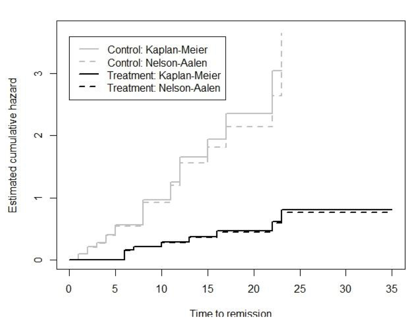
圖 86.6: Leukaemia patient data: comparing Kaplan-Meier and Nelson-Aalen estimates of the cumulative hazard in the treatment and control groups.
86.8 關於非參數分析法的一些延伸
目前本章節的例子主要關注了兩組之間的生存曲線的比較,但是很顯然它可以被擴展開去:
- 非參數法比較生存曲線也可以用於比較2組以上的生存曲線。
- 如果有一些我們希望能夠控制的變量恰好是分類型的變量(例如性別),那麼我們可以依據該非類型數據繪製每個分類的生存曲線進行視覺上的比較。
- 很顯然當你有許多個分類變量需要進行調整的時候,2. 的方法就顯得過於耗時耗力。
- 非參數法分析生存數據最明顯的缺陷是,使用非參數法我們只能進行粗略且無法定量的比較。也就是說當治療組與對照組存在生存曲線的差異時,我們沒辦法定量地描述其差異是多少。
- 另外,非參數法分析生存數據的另一個缺點是,這種手段對連續型的暴露變量其實是束手無策的。某些情況下可能可以把連續變量人爲地分割成一個分類型變量,但這顯然並不能令人滿意。
86.9 Practical Survival 02
86.9.1 Part 1: PBC 數據
- 在R裏讀入數據,熟悉數據的各個變量,哪個變量是用於表示事件發生與否的指示變量(failure indicator)?哪些變量又表示患者進入/離開研究的時間點?哪個變量表示了患者的治療組?總結(summary)兩個治療組的生存時間。
# summarize and explore the data
library(haven)
pbcbase <- read_dta("../backupfiles/pbcbase.dta")
head(pbcbase)
## # A tibble: 6 × 17
## id datein dateout time d treat age logb0c alb0c logigm0c cenc0 cir0 gh0 asc0
## <dbl> <date> <date> <dbl> <dbl> <dbl> <dbl> <dbl> <dbl> <dbl> <dbl> <dbl> <dbl> <dbl>
## 1 5 1980-02-19 1981-09-19 1.58 1 1 46 1.04 -2.52 -8.80e-1 1 0 0 0
## 2 22 1980-08-22 1980-08-22 0 0 2 68 0.400 6.68 7.90e-1 0 1 0 0
## 3 23 1980-07-22 1989-08-02 9.03 0 2 65 0.0800 7.68 1.60e-1 0 0 0 0
## 4 40 1980-08-08 1982-11-21 2.29 1 1 36 0.400 4.68 7.00e-2 0 1 0 0
## 5 42 1980-09-06 1982-10-05 2.08 1 1 38 0.830 4.68 -1.19e-9 0 0 0 1
## 6 45 1980-02-09 1985-06-02 5.31 1 1 48 -0.260 5.68 -8.40e-1 1 0 0 0
## # … with 3 more variables: bil0 <dbl>, alb0 <dbl>, igm0 <dbl>##
## Original table
## d
## treat 0 1 Total
## 1 45 49 94
## 2 50 47 97
## Total 95 96 191
##
## Row percent
## d
## treat 0 1 Total
## 1 45 49 94
## (47.9) (52.1) (100)
## 2 50 47 97
## (51.5) (48.5) (100)
##
## Column percent
## d
## treat 0 % 1 %
## 1 45 (47.4) 49 (51)
## 2 50 (52.6) 47 (49)
## Total 95 (100) 96 (100)## treat d Median
## 1 1 0 3.7426419
## 2 1 1 3.0006845
## 3 2 0 5.4483230
## 4 2 1 2.2012320- 你能親手計算下面不完整表格中的?部分嗎?
| Time | Beg. Total | Fail | Net Lost | Survivor Function |
|---|---|---|---|---|
| 0.104 | 26 | 1 | 0 | 0.9615 |
| 0.2628 | 25 | 1 | 0 | 0.9231 |
| 0.4572 | 24 | 1 | 0 | 0.8846 |
| 0.4846 | 23 | 1 | 0 | 0.8462 |
| 0.9172 | 22 | 0 | 1 | 0.8462 |
| 1.164 | 21 | 1 | 0 | 0.8059 |
| 1.369 | 20 | 1 | 0 | 0.7656 |
| 1.572 | 19 | 0 | 1 | ? |
| 1.687 | 18 | 1 | 0 | ? |
| 1.725 | 17 | 1 | 0 | ? |
| 2.182 | 16 | 1 | 0 | ? |
| 2.201 | 15 | 1 | 0 | 0.5954 |
| 2.634 | 14 | 0 | 1 | ? |
| 2.667 | 13 | 1 | 0 | ? |
| 3.047 | 12 | 0 | 1 | 0.5496 |
| 3.45 | 11 | 1 | 0 | 0.4997 |
| … | … | … | … | … |
| 8.89 | 2 | 0 | 1 | 0.1399 |
| 11.25 | 1 | 0 | 1 | 0.1399 |
正確答案在這裏,你算對了嗎?
           Beg.          Net            Survivor      Std.
  Time    Total   Fail   Lost           Function     Error     [95% Conf. Int.]
-------------------------------------------------------------------------------
  .104       26      1      0             0.9615    0.0377     0.7569    0.9945
 .2628       25      1      0             0.9231    0.0523     0.7260    0.9802
 .4572       24      1      0             0.8846    0.0627     0.6836    0.9613
 .4846       23      1      0             0.8462    0.0708     0.6404    0.9393
 .9172       22      0      1             0.8462    0.0708     0.6404    0.9393
 1.164       21      1      0             0.8059    0.0780     0.5946    0.9143
 1.369       20      1      0             0.7656    0.0839     0.5505    0.8873
 1.572       19      0      1             0.7656    0.0839     0.5505    0.8873
 1.687       18      1      0             0.7230    0.0894     0.5044    0.8576
 1.725       17      1      0             0.6805    0.0937     0.4603    0.8262
 2.182       16      1      0             0.6380    0.0970     0.4180    0.7933
 2.201       15      1      0             0.5954    0.0994     0.3773    0.7590
 2.634       14      0      1             0.5954    0.0994     0.3773    0.7590
 2.667       13      1      0             0.5496    0.1018     0.3337    0.7215
 3.047       12      0      1             0.5496    0.1018     0.3337    0.7215
  3.45       11      1      0             0.4997    0.1041     0.2866    0.6803
 3.472       10      1      0             0.4497    0.1050     0.2425    0.6371
 3.855        9      1      0             0.3997    0.1045     0.2012    0.5920
 4.249        8      1      0             0.3498    0.1027     0.1625    0.5448
  5.47        7      0      1             0.3498    0.1027     0.1625    0.5448
 5.541        6      0      1             0.3498    0.1027     0.1625    0.5448
 6.762        5      1      0             0.2798    0.1033     0.1056    0.4859
 6.905        4      1      0             0.2099    0.0983     0.0601    0.4202
 8.019        3      1      0             0.1399    0.0869     0.0259    0.3469
  8.89        2      0      1             0.1399    0.0869     0.0259    0.3469
 11.25        1      0      1             0.1399    0.0869     0.0259    0.3469
-------------------------------------------------------------------------------## Call: survfit(formula = Surv(time, d) ~ treat, data = pbcbase)
##
## treat=1
## time n.risk n.event survival std.err lower 95% CI upper 95% CI
## 0.02464 90 1 0.9889 0.01105 0.96747 1.0000
## 0.05202 89 1 0.9778 0.01554 0.94779 1.0000
## 0.10404 88 1 0.9667 0.01892 0.93028 1.0000
## 0.13142 87 1 0.9556 0.02172 0.91391 0.9991
## 0.41068 86 1 0.9444 0.02415 0.89829 0.9930
## 0.67077 84 1 0.9332 0.02635 0.88297 0.9863
## 0.70089 83 1 0.9220 0.02833 0.86808 0.9792
## 0.93361 81 1 0.9106 0.03018 0.85331 0.9717
## 1.08145 79 1 0.8990 0.03192 0.83861 0.9638
## 1.21287 77 1 0.8874 0.03357 0.82395 0.9557
## 1.24846 76 1 0.8757 0.03510 0.80953 0.9473
## 1.25120 75 1 0.8640 0.03653 0.79532 0.9387
## 1.32512 74 1 0.8523 0.03785 0.78129 0.9299
## 1.42916 73 1 0.8407 0.03909 0.76744 0.9209
## 1.45927 72 1 0.8290 0.04026 0.75373 0.9118
## 1.46475 71 1 0.8173 0.04135 0.74017 0.9025
## 1.58248 70 1 0.8056 0.04237 0.72673 0.8931
## 2.07803 66 1 0.7934 0.04345 0.71268 0.8833
## 2.28611 64 1 0.7810 0.04451 0.69850 0.8733
## 2.63655 63 1 0.7686 0.04550 0.68445 0.8632
## 2.80082 61 1 0.7560 0.04646 0.67025 0.8528
## 2.80356 60 1 0.7434 0.04737 0.65617 0.8423
## 2.89117 58 1 0.7306 0.04825 0.64191 0.8316
## 2.90212 57 1 0.7178 0.04908 0.62778 0.8207
## 3.00068 56 1 0.7050 0.04985 0.61375 0.8098
## 3.25530 51 1 0.6912 0.05075 0.59852 0.7981
## 3.29090 50 1 0.6773 0.05158 0.58342 0.7864
## 3.33196 49 1 0.6635 0.05235 0.56845 0.7745
## 4.18344 43 1 0.6481 0.05336 0.55150 0.7616
## 4.27105 42 1 0.6327 0.05427 0.53474 0.7485
## 4.33676 41 1 0.6172 0.05510 0.51815 0.7352
## 4.55852 40 1 0.6018 0.05584 0.50172 0.7218
## 4.63518 38 1 0.5860 0.05657 0.48493 0.7080
## 4.77481 36 1 0.5697 0.05730 0.46776 0.6938
## 4.87611 34 1 0.5529 0.05801 0.45016 0.6792
## 4.93635 33 1 0.5362 0.05862 0.43275 0.6643
## 4.99658 31 1 0.5189 0.05923 0.41486 0.6490
## 5.14990 30 1 0.5016 0.05972 0.39718 0.6334
## 5.27584 28 1 0.4837 0.06022 0.37894 0.6173
## 5.31143 27 1 0.4658 0.06059 0.36092 0.6010
## 5.40726 26 1 0.4478 0.06085 0.34313 0.5845
## 6.05613 19 1 0.4243 0.06205 0.31853 0.5651
## 6.20671 18 1 0.4007 0.06292 0.29455 0.5451
## 6.41478 16 1 0.3757 0.06378 0.26933 0.5240
## 6.92950 12 1 0.3443 0.06570 0.23692 0.5005
## 6.94593 11 1 0.3130 0.06677 0.20609 0.4755
## 7.12663 8 1 0.2739 0.06894 0.16725 0.4486
## 7.78371 6 1 0.2283 0.07097 0.12410 0.4199
## 9.25941 2 1 0.1141 0.08816 0.02511 0.5187
##
## treat=2
## time n.risk n.event survival std.err lower 95% CI upper 95% CI
## 0.02464 93 1 0.9892 0.01069 0.9685 1.0000
## 0.10404 92 1 0.9785 0.01504 0.9495 1.0000
## 0.26283 91 1 0.9677 0.01832 0.9325 1.0000
## 0.39425 90 1 0.9570 0.02104 0.9166 0.9991
## 0.45722 89 1 0.9462 0.02339 0.9015 0.9932
## 0.48460 88 1 0.9355 0.02547 0.8869 0.9868
## 0.52841 86 1 0.9246 0.02740 0.8724 0.9799
## 0.55031 85 1 0.9137 0.02916 0.8583 0.9727
## 0.56674 84 1 0.9029 0.03077 0.8445 0.9652
## 0.68720 83 1 0.8920 0.03227 0.8309 0.9575
## 1.15264 79 1 0.8807 0.03378 0.8169 0.9494
## 1.16359 78 1 0.8694 0.03518 0.8031 0.9412
## 1.27036 77 1 0.8581 0.03649 0.7895 0.9327
## 1.36893 75 1 0.8467 0.03776 0.7758 0.9240
## 1.60438 72 1 0.8349 0.03902 0.7618 0.9150
## 1.68652 71 1 0.8231 0.04020 0.7480 0.9058
## 1.72485 70 1 0.8114 0.04131 0.7343 0.8965
## 1.74127 69 1 0.7996 0.04235 0.7208 0.8871
## 1.77139 68 1 0.7879 0.04333 0.7073 0.8775
## 1.88364 66 1 0.7759 0.04429 0.6938 0.8678
## 2.03422 65 1 0.7640 0.04519 0.6804 0.8579
## 2.06434 64 1 0.7521 0.04603 0.6670 0.8479
## 2.18207 62 1 0.7399 0.04686 0.6535 0.8377
## 2.20123 60 1 0.7276 0.04768 0.6399 0.8273
## 2.59274 56 1 0.7146 0.04856 0.6255 0.8164
## 2.66667 54 1 0.7014 0.04943 0.6109 0.8053
## 3.33744 52 1 0.6879 0.05029 0.5960 0.7939
## 3.41410 51 1 0.6744 0.05108 0.5814 0.7823
## 3.44969 50 1 0.6609 0.05181 0.5668 0.7707
## 3.47159 49 1 0.6474 0.05248 0.5523 0.7589
## 3.85489 47 1 0.6336 0.05314 0.5376 0.7468
## 4.10404 45 1 0.6196 0.05379 0.5226 0.7345
## 4.10678 44 1 0.6055 0.05438 0.5077 0.7220
## 4.16701 43 1 0.5914 0.05491 0.4930 0.7094
## 4.24914 42 1 0.5773 0.05538 0.4784 0.6967
## 4.25462 41 1 0.5632 0.05579 0.4639 0.6839
## 5.31691 37 1 0.5480 0.05632 0.4480 0.6703
## 5.40726 36 1 0.5328 0.05677 0.4324 0.6565
## 5.88090 28 1 0.5138 0.05785 0.4120 0.6406
## 6.04791 27 1 0.4947 0.05875 0.3920 0.6244
## 6.64203 21 1 0.4712 0.06049 0.3664 0.6060
## 6.76249 19 1 0.4464 0.06218 0.3397 0.5865
## 6.84463 17 1 0.4201 0.06383 0.3119 0.5658
## 6.90486 16 1 0.3939 0.06502 0.2850 0.5443
## 7.82204 13 1 0.3636 0.06670 0.2538 0.5209
## 8.01917 12 1 0.3333 0.06768 0.2238 0.4962
## 8.27926 11 1 0.3030 0.06797 0.1952 0.4703plot(pbc.km, conf.int = F, col = c("red", "black"), mark.time = F, xlab = "Time", ylab = "Survivor function")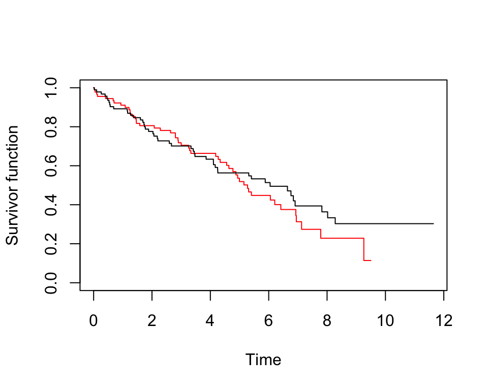
圖 86.7: Rplots of the Kaplan-Meier survivor functions
plot(pbc.km, conf.int = T, col = c("red", "black"), mark.time = T, xlab = "Time", ylab = "Survivor function")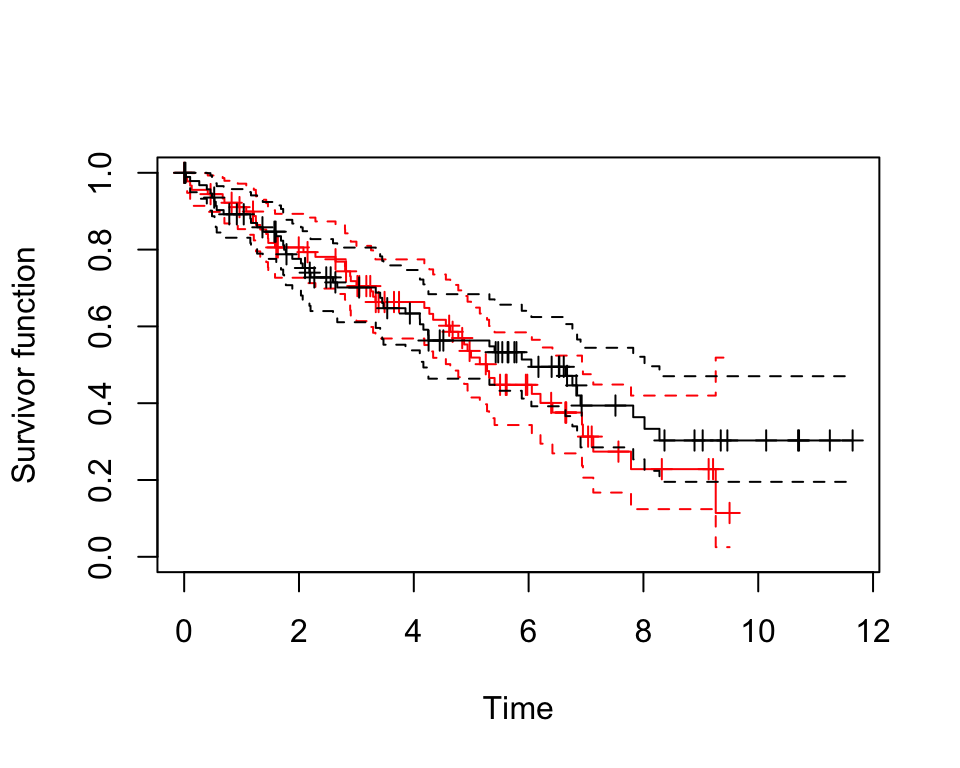
圖 86.8: Rplots of the Kaplan-Meier survivor functions with confidence intervals
在追蹤前兩年,兩組患者的生存方程沒有太大區別,兩年之後,到大約第五年之間,藥物治療組的生存概率曲線似乎要低於對照組,暗示藥物治療在這段時間內可能導致患者較高的死亡率。患者隨訪達到第五年之後,可以看到藥物治療組患者的生存概率曲線一直都處在對照組的上方,提示我們患者被隨訪達到五年之後,藥物治療組的患者死亡率開始低於對照組死亡率。但是,這兩條生存概率曲線的 95% 信賴區間彼此重疊部分很大,且在臨近隨訪達到12年的時候,信賴區間太寬,因爲此時已經沒有多少死亡病例。這兩組患者都有大約 50% 左右的患者的生存率超過五年。
pbc.km1 <- survfit(Surv(time, d) ~ 1, data=subset(pbcbase, pbcbase$treat == 1))
pbc.km2 <- survfit(Surv(time, d) ~ 1, data=subset(pbcbase, pbcbase$treat == 2))
cumhaz.1 <- cumsum(pbc.km1$n.event/pbc.km1$n.risk)
cumhaz.2 <- cumsum(pbc.km2$n.event/pbc.km2$n.risk)
plot(pbc.km1$time, cumhaz.1, type = "s", col = "red", xlab = "Time", ylab = "Cumulative hazard")
lines(pbc.km2$time, cumhaz.2, type = "s", col = "black")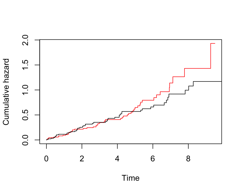
圖 86.9: Rplots of the Nelson-Aalen estimates of the cumulative hazard
plot(pbc.km, conf.int= F, col=c("red", "black"), mark.time =F,xlab = "Time", ylab = "Cumulative hazard", fun = "cumhaz")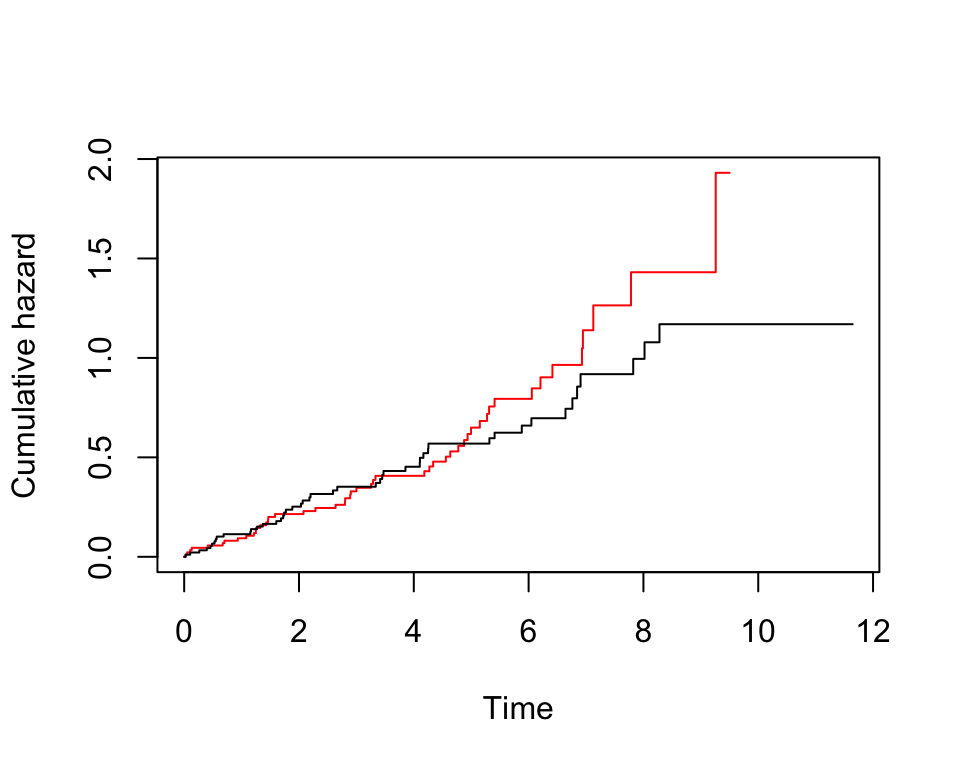
圖 86.10: Rplots of the Kaplan-Meier estimates of the cumulative hazard
從兩個生存累積概率曲線來看,治療組的生存累計概率似乎隨着時間更加呈線性變化。在對照組,風險在5年以後的累計速率陡然升高了。
## Call:
## survdiff(formula = Surv(time, d) ~ treat, data = pbcbase)
##
##          N Observed Expected (O-E)^2/E (O-E)^2/V
## treat=1 94       49    45.33    0.2966    0.5696
## treat=2 97       47    50.67    0.2654    0.5696
##
##  Chisq= 0.6  on 1 degrees of freedom, p= 0.45
whitehall <- read_dta("../backupfiles/whitehall.dta")
whl.km <- survfit(Surv(time=(timeout - timein)/365.25, event = chd) ~ 1, data = whitehall)
plot(whl.km, conf.int = T, mark.time = F, xlab = "Time", ylab = "Survivor function", ylim=c(0.8,1))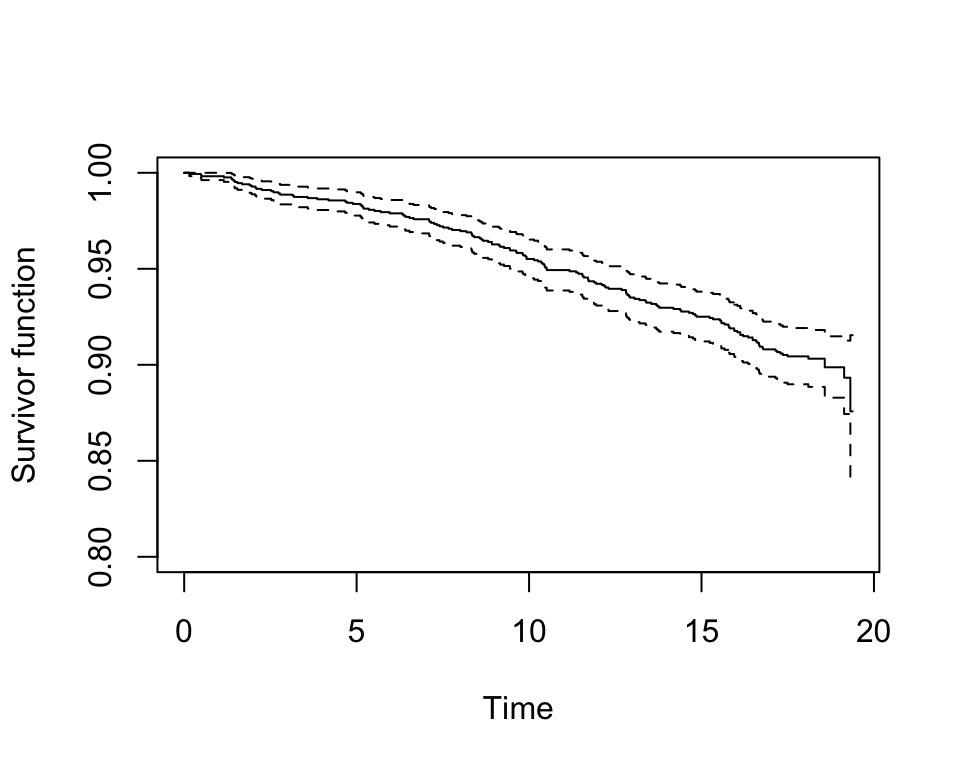
圖 86.11: Rplots of the Kaplan-Meier estimates of the survivor curve
whl.km <- survfit(Surv(time = (timeout - timein)/365.25, event = chd) ~ sbpgrp, data = whitehall)
plot(whl.km, conf.int = F, mark.time = F, xlab = "Time", ylab = "Survivor function", ylim = c(0.75, 1), col = c("blue", "red", "green", "orange"))
legend(1, 0.85, c("Group 1", "Group 2", "Group 3", "Group 4"), col = c("blue", "red", "green", "orange"), lty = c(1,1))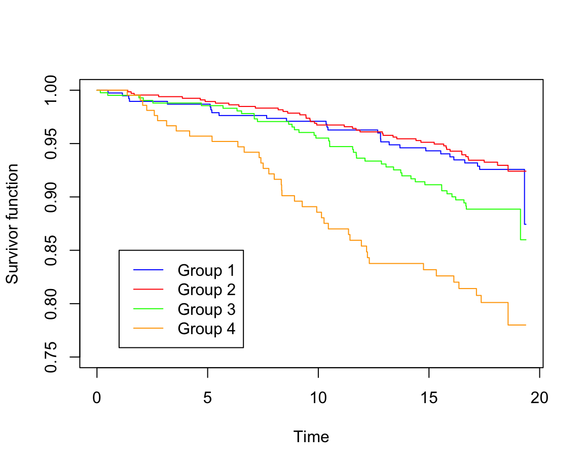
圖 86.12: Rplots of the Kaplan-Meier estimates of the survivor curve
所以,第四組患者的生存率最差, 第一組,第二組患者幾乎沒有差別。
## Call:
## survdiff(formula = Surv(time = (timeout - timein)/365.25, event = chd) ~
##     sbpgrp, data = whitehall)
##
##            N Observed Expected (O-E)^2/E (O-E)^2/V
## sbpgrp=1 383       28    36.81    2.1101     2.776
## sbpgrp=2 664       44    62.90    5.6786     9.602
## sbpgrp=3 417       43    37.09    0.9411     1.240
## sbpgrp=4 213       39    17.20   27.6494    31.153
##
##  Chisq= 36.4  on 3 degrees of freedom, p= 6.1e-08