第 76 章 縱向研究數據 longitudinal data 1
本章我們來把目前爲止了解的混合效應 (截距/斜率) 模型應用到一種特殊形態的數據 – 縱向研究數據 – 中去。
縱向數據,是一種前瞻性收集的來的數據,它隨着時間的推移,在不同的時間點對相同的觀察對象進行數據的採集。每個研究對象被收集數據時的時間點,可以是相同的,也可以是不同的。在很多臨牀實驗中,患者被觀察隨訪,並且常常在同樣的時間點收集數據,所以在臨牀實驗的特殊形態下,每個患者收集數據的時間點可以做到統一,這樣的縱向研究數據是屬於固定測量時刻的類型 (fixed occasions)。但是在流行病學等觀察性研究中獲得的數據,就沒有這麼幸運,他們通常測量收集數據的時間點就不太可能保持一致,收集時間點不一致的縱向數據屬於不固定測量時刻的類型 (variable occasions)。
縱向數據英文名是 longitudinal data,它的常見別的名稱是 重復測量數據 (repeated measures data),計量經濟學中叫做面板型數據 (panel data),或者是時間序列橫斷面研究數據 (cross sectional time series data)。所以在縱向數據這種特殊形態的的嵌套式數據結構中,第二層級結構就是一個個的個體,第一層級結構,就是每個個體在不同的時間點獲得的測量值。除了和前面幾章討論過的嵌套式數據結構相似可以應用混合效應模型,縱向數據還有一些自己獨特的性質需要加以考量:
- 層內數據的相關性結構是有測量時間的先後順序的;
- 之前討論的嵌套式結構數據在層內的觀察值則沒有嚴格的時間或者大小的排序 (例如同一所學校的不同學生);
- 換句話說,層內相關系數 (intra-class correlation) 很難被認爲是相似或者相同的。
76.1 固定測量時刻 fixed occasions
對於臨牀試驗中固定時刻隨訪收集到的病人數據,理想狀態下應該是一種平衡數據 (balanced data)。也就是在不同時間 \(t_i , i = 1, \cdots, n\) 我們成功收集到所有患者的所有數據,所以每層 (名患者) 擁有的時間序列數據的樣本量是相同的 \(n_j = n, \forall j\)。
如同分析其他類型的數據一樣,分析縱向數據也要從描述數據開始。如果是平衡數據,描述性分析就很容易,當有缺失值時,分析就變得有些棘手。例如,我們可以計算每個時間點的平均值作爲所有患者的 “平均特質 average profiles”。或者也可以用每個人的時間序列數據對時間做簡單線性回歸模型,從而獲取每個個體的截距和斜率。
76.1.1 缺失值 Missing data
當縱向數據中存在一些缺失值,即使你在計算一些簡單的歸納性分析,也要特別特別特別地小心。如果不是所有人都有全部測量時間點的數據的話,總體的平均特徵數據分析了也沒有太大的卵用,因爲缺失值導致這樣計算獲得的並不是真實的平均值 (也因爲不同的患者,貢獻了不同時間點的數據,沒辦法平均)。
如果存在缺失值,那麼當且僅當這些缺失值和觀測值 \(Y\) 之間沒有關系時,才能認爲這些簡單計算和簡單模型的建立是不帶有偏倚的。如果說,有些缺失值確實是根據觀測數據有選擇性地缺失 (the mechanism driving the selection depends on measured data),隨機效應模型的建立可以自動化校正這樣的缺失,從而保證估計無偏。
根據觀測數據選擇性地出現缺失值的機制被叫做隨機缺失 (Missing at random, MAR)。
76.1.1.1 隨機截距模型 random intercept model
復合對稱模型 compound symmetry model, 是常見的一種用於重復測量數據的模型,它是基於隨機截距模型的一種擴展模型。
當模型中沒有解釋變量時,
\[ \begin{equation} Y_{ij} = \mu_i + u_{0j} + e_{ij} \end{equation} \tag{76.1} \]
其中,
- \(i\) 是測量時刻;
- \(j\) 是實驗的個體;
- \(\mu_i\) 是測量時刻 \(i\) 時的平均截距 – 這是一個固定效應。
爲了擬合這個模型,我們需要先生成一系列的啞變量用來表示不同的測量時刻:
\[ Y_{ij} = \sum_{h=1}^n\beta_{0h} I_{i = h,j} + u_{0j} + e_{ij} \]
其中,
- \(I_{i = h,j}\) 是用於表示第 \(j\) 名患者的 \(i\) 次觀測值,在第 \(h\) 次測量時是否被測量到的啞變量。
- 該模型暗示同一個患者收集到的不同時刻的觀察數據是可以互換的,有相同的協方差 \[ \begin{aligned} \text{Cov}(Y_{1j} , Y_{2j}) & = \text{Cov}(u_{0j} + e_{1j}, u_{0j} + e_{2j}) \\ & = \sigma^2_{u_{00}} \end{aligned} \]
- 該模型還有另一個暗示是,不同患者之間任意時間點的兩個觀察數據之間是相互獨立的 \[ \begin{aligned} \text{Cov}(Y_{1j}, Y_{2j*}) & = \text{Cov}(u_{0j} + e_{1j}, u_{0j*} + e_{2j*}) \\ & = 0 \end{aligned} \]
所以當沒有缺失值時,數據是固定測量時刻 (fixed occation) 的數據也是是平衡數據,那麼每一個患者 (第二層級數據) 的觀察值可以寫作是一個向量 \(\{ \mathbf{Y}_{ij} \}\),每名患者的觀察值向量的長度都是相同的 \(n\)。所以,它們的 \(n\times n\) 協方差矩陣就是:
\[ \Omega_y = \left( \begin{array}{cccc} \sigma^2_{u_{00}} + \sigma^2_e & \sigma^2_{u_{00}} & \cdots & \sigma^2_{u_{00}} \\ \sigma_{u_{00}} & \sigma^2_{u_{00}} + \sigma^2_e & \cdots & \sigma^2_{u_{00}} \\ \vdots & \vdots & \vdots & \vdots \\ \sigma^2_{u_{00}} & \sigma^2_{u_{00}} & \cdots & \sigma^2_{u_{00}} + \sigma^2_e\\ \end{array} \right) \]
也正是由於觀測值的協方差矩陣是如此地對稱,該模型被命名爲復合對稱模型 compound symmetric model。
Adult height measures 數據
有(閒人)花了數十年時間追蹤隨訪了近2000名女性在 26 歲,36歲,43歲,53歲時的身高。忽略掉可能存在的測量誤差,研究者想知道是否隨着年齡增加,女性的身高會縮水。這些女性在這些年齡時的身高數據總結如下:
##
## No. of observations = 2187
##
##   Var. name obs. mean   median  s.d.   min.   max.
## 1 ht26      1758 162.33 162.6   6.36   142.2  180.3
## 2 ht36      1610 162.26 162.2   6.05   135.2  180
## 3 ht43      1567 162.28 162.1   5.96   140    180
## 4 ht53      1462 161.56 161.5   5.96   134.3  179.6
原則上每個女性在所有的時間應該都有身高測量值才對,我們暫且認爲擁有缺失測量值的時間點是完全隨機的。先計算樣本中數據完整部分的女性身高在四個時間點時的方差協方差矩陣:
##           ht26      ht36      ht43      ht53
## ht26 39.813400 34.758457 34.478981 34.128167
## ht36 34.758457 34.455060 33.360413 33.086680
## ht43 34.478981 33.360413 34.331501 32.948850
## ht53 34.128167 33.086680 32.948850 34.215187
要給這個數據擬合混合對稱模型 (compound symmetry model),需要先把數據從寬變長,之後爲每個測量身高的時間點生成一個啞變量,然後擬合無截距式的隨機截距模型:
# 把數據格式從寬變長
hei_long <- height %>%
  gather(key, value, -id, -bw, -mht) %>%
    separate(key, into = c("Height", "H_Age"), sep = 2) %>%
      arrange(id, H_Age, bw, mht) %>%
        spread(Height, value)

# 生成四個年齡時間點數據的啞變量
hei_long <- hei_long %>%
  mutate(Age_1 = ifelse(H_Age == 26, 1, 0),
         Age_2 = ifelse(H_Age == 36, 1, 0),
         Age_3 = ifelse(H_Age == 43, 1, 0),
         Age_4 = ifelse(H_Age == 53, 1, 0))
M_hei <- lmer(ht ~ 0 + Age_1 + Age_2 + Age_3 + Age_4 + (1 | id), data = hei_long, REML = TRUE)
summary(M_hei)
## Linear mixed model fit by REML. t-tests use Satterthwaite's method ['lmerModLmerTest']
## Formula: ht ~ 0 + Age_1 + Age_2 + Age_3 + Age_4 + (1 | id)
## Data: hei_long
##
## REML criterion at convergence: 30475.2
##
## Scaled residuals:
## Min 1Q Median 3Q Max
## -4.69990 -0.46089 -0.00475 0.45917 8.26749
##
## Random effects:
## Groups Name Variance Std.Dev.
## id (Intercept) 35.9056 5.9921
## Residual 1.9862 1.4093
## Number of obs: 6397, groups: id, 1980
##
## Fixed effects:
## Estimate Std. Error df t value Pr(>|t|)
## Age_1 162.34141 0.13903 2151.19110 1167.7 < 2.2e-16 ***
## Age_2 162.31738 0.13977 2195.10604 1161.3 < 2.2e-16 ***
## Age_3 162.19431 0.13997 2207.43546 1158.8 < 2.2e-16 ***
## Age_4 161.45320 0.14041 2234.23200 1149.9 < 2.2e-16 ***
## ---
## Signif. codes: 0 '***' 0.001 '**' 0.01 '*' 0.05 '.' 0.1 ' ' 1
##
## Correlation of Fixed Effects:
## Age_1 Age_2 Age_3
## Age_2 0.933
## Age_3 0.931 0.933
## Age_4 0.928 0.930 0.931# 檢驗三個年齡點的身高均值是否相同用下面的方法:
linearHypothesis(M_hei, c("Age_1 - Age_2 = 0",
"Age_1 - Age_3 = 0",
"Age_1 - Age_4 = 0"))## Linear hypothesis test
##
## Hypothesis:
## Age_1 - Age_2 = 0
## Age_1 - Age_3 = 0
## Age_1 - Age_4 = 0
##
## Model 1: restricted model
## Model 2: ht ~ 0 + Age_1 + Age_2 + Age_3 + Age_4 + (1 | id)
##
## Df Chisq Pr(>Chisq)
## 1
## 2 3 374.564 < 2.22e-16 ***
## ---
## Signif. codes: 0 '***' 0.001 '**' 0.01 '*' 0.05 '.' 0.1 ' ' 1所以,用這個模型 (符合對稱模型 compound symmetry model),其實我是在告訴 R 軟件說,我認爲,這個數據中的女性四次測量的身高之間的方差協方差矩陣是這樣紙的 (因爲 \(5.992^2 = 35.91; 1.409^2 = 1.99\)):
\[ \Omega_y = \left( \begin{array}{cccc} 37.90 & 35.91 & 35.91 & 35.91 \\ 35.91 & 37.90 & 35.91 & 35.91 \\ 35.91 & 35.91 & 37.90 & 35.91 \\ 35.91 & 35.91 & 35.91 & 37.90\\ \end{array} \right) \]
分析這個模型第二層階級殘差,和第一層階級殘差可以計算並做圖 76.1 76.2 如下:
# refit the model with lme
M_hei <- lme(fixed = ht ~ 0 + Age_1 + Age_2 + Age_3 + Age_4, random = ~ 1 | id,
             data = hei_long, method = "REML", na.action=na.omit)
# individual level standardized residuals
ehat_st <- residuals(M_hei, type = "normalized", level = 1)

# extract the EB uhat (level 2 EB residual)
uhat_eb <- ranef(M_hei)$`(Intercept)`

# standardized level 2 residuals
### count number of measures for each women
Nmeas <- 4
### shrinkage factor
R = 5.992^2/(5.992^2 + 1.409^2/Nmeas)
### use shrinkage factor calculate variance of uhat_eb
var_eb <- R * 5.992^2
### standardize uhat
uhat_st <- uhat_eb/sqrt(var_eb)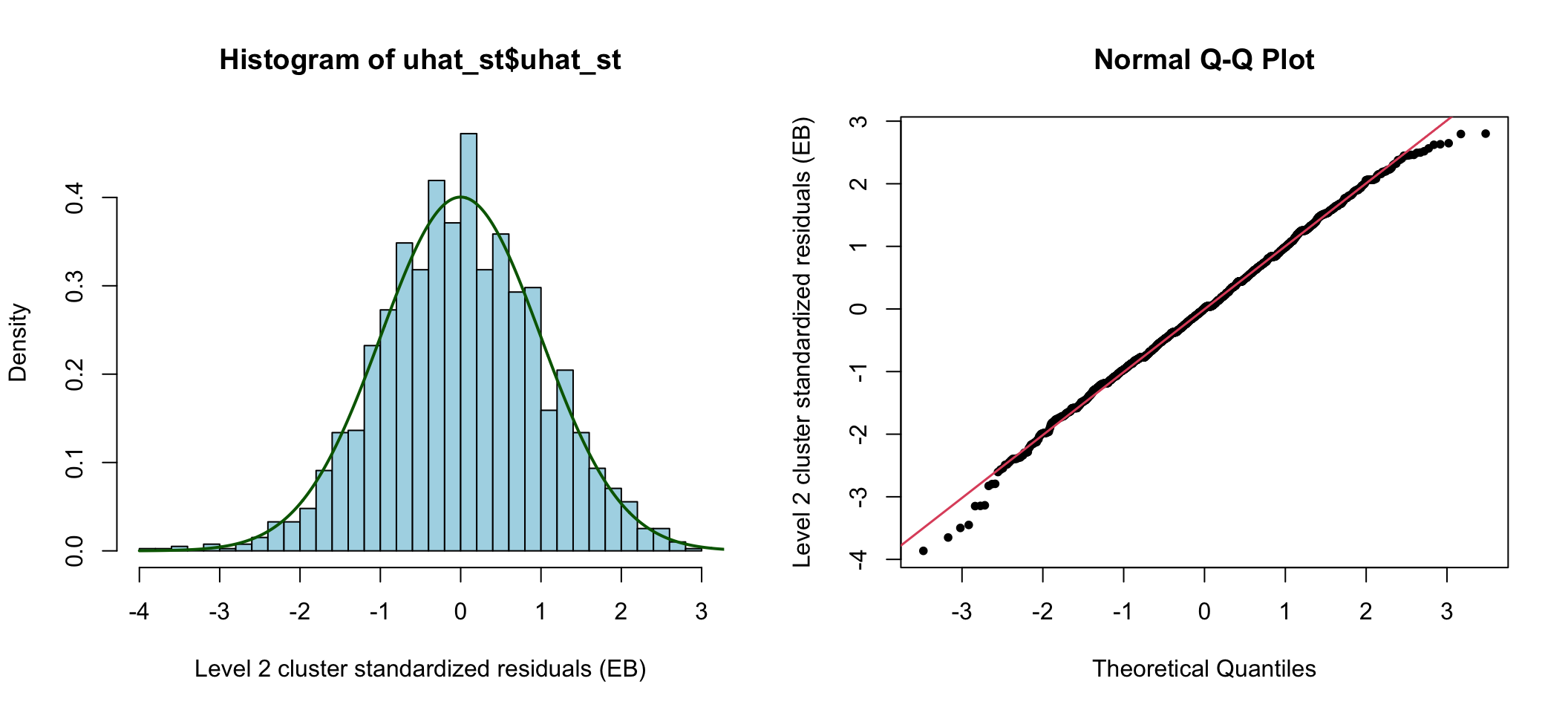
圖 76.1: Standardized cluster level residuals (intercept) from the compound symmetry model
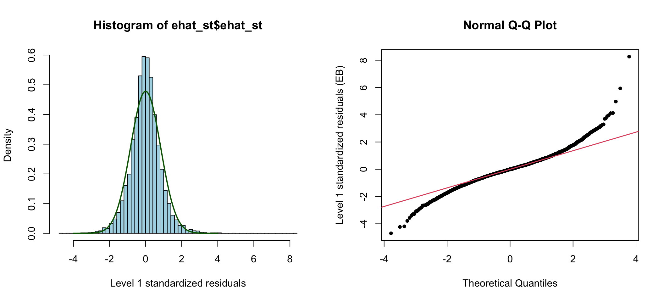
圖 76.2: Standardized elementary level residuals from the compound symmetry model
混合對稱模型的前提假設實在是太強了 (它假定個體內的方差保持不變,且個體間的協方差也保持不變)。你我都清楚,當考慮了時間以後,同一個體在時間上比較接近的點測量之間會更相似,也更相關。
76.1.1.2 隨機參數模型 random intercept and slope model
實際上有多種方法可以放鬆混合對稱模型對方差和協方差的約束性前提,其中之一是在隨機截距模型中允許有隨機斜率成分。
使用隨機參數模型擬合縱向數據時的簡單模型如下:
\[ Y_{ij} = (\beta_0 + u_{0j}) + (\beta_1 + u_{1j})t_i +e_{ij} \]
前一章討論過 (滾回 75.5),這裏隨機參數模型的解釋變量是時間 \(t_i\),導致的結果之一是觀測值的方差其實是隨着時間變化而變化的 (拋物線關系):
\[ \begin{aligned} \text{Var}(Y_{ij}) & = \text{Cov}(u_{0j} + u_{ij}t_i + e_{ij}, u_{0j} + u_{ij}t_i + e_{ij}) \\ & = \sigma^2_{u_{00}} + \sigma^2_{u_{11}}t_i^2 + 2t_i\sigma_{u_{01}} + \sigma^2_e \end{aligned} \]
同時,同一患者不同時間測量的觀測值之間的協方差是:
\[ \begin{aligned} \text{Cov}(Y_{1j}, Y_{2j}) & = \text{Cov}(u_{0j} + u_{1j}t_1 + e_{1j}, u_{0j} + u_{2j}t_2 + e_{2j}) \\ & = \sigma^2_{u_{00}} + \sigma^2_{u_{11}}t_1t_2 + \sigma_{u_{01}}(t_1 + t_2) \end{aligned} \]
不同患者任意測量時刻之間的協方差是:
\[ \begin{aligned} \text{Cov}(Y_{1j}, Y_{2j*}) & = \text{Cov}(u_{0j} + u_{1j}t_1 + e_{1j}, u_{0j*} + u_{2j*}t_2 + e_{2j*}) \\ & = 0 \end{aligned} \]
Adult height measures 數據
利用上面的理論,來對身高數據擬合另一個混合效應模型:
# 對年齡中心化到以 26 歲爲起點
hei_long <- hei_long %>%
  mutate(age = as.numeric(H_Age) - 26)
M_hei_ran <- lme(fixed = ht ~ age, random = ~ age | id, data = hei_long, method = "REML", na.action = na.omit)
#M_hei_ran <- lmer(ht ~ age + (age | id), data = hei_long, REML = TRUE)
summary(M_hei_ran)
## Linear mixed-effects model fit by REML
## Data: hei_long
## AIC BIC logLik
## 30382.427 30423.006 -15185.213
##
## Random effects:
## Formula: ~age | id
## Structure: General positive-definite, Log-Cholesky parametrization
## StdDev Corr
## (Intercept) 6.158844461 (Intr)
## age 0.059929577 -0.281
## Residual 1.259210715
##
## Fixed effects: ht ~ age
## Value Std.Error DF t-value p-value
## (Intercept) 162.49616 0.141129788 4416 1151.39521 0
## age -0.03158 0.002273653 4416 -13.88951 0
## Correlation:
## (Intr)
## age -0.279
##
## Standardized Within-Group Residuals:
## Min Q1 Med Q3 Max
## -3.9386997037 -0.4542383377 -0.0066047395 0.4297466693 5.5051619208
##
## Number of Observations: 6397
## Number of Groups: 1980這個混合效應模型同時包含了隨機截距和隨機斜率兩個部分。你可以用 LRT 比較它和一個只有隨機截距的模型哪個更好,但是我們沒有辦法比較它和混合對稱模型哪個更優於擬合這個數據 (因爲他們的固定效應部分不同,在 REML 方法下實際二者擬合的數據是不同的)。這個隨機系數模型和前一個混合對稱模型都給出了身高隨着年齡增加而減少的相同結論。不同的是,隨機系數模型把同一對象內不同時間觀測值之間的等協方差的約束條件給放開了,因爲用腳趾頭想也知道同一個人不同時間測量的數據之間的協方差會隨着時間跨度不同而發生改變。
根據隨機系數模型給出的報告,計算模型估計的觀測值 (身高的4個時間點) 的方差協方差矩陣:
\[ \begin{aligned} \hat{\text{Cov}}(Y_{1j}, Y_{2j}) & = \sigma^2_{u_{00}} + \sigma^2_{u_{11}}t_1t_2 +\sigma_{u_{01}} (t_1 + t_2) \\ & = 6.1588^2 + 0.0599^2t_1t_2 + (-0.28)\times6.1588\times0.0599 (t_1 + t_2)\\ & = 37.93 + 0.004\times t_2 \times t_2 - 0.104 \times(t_1 + t_2) \\ \hat{\text{Var}} (Y_1j) & = \sigma^2_{u_{00}} + \sigma^2_{u_{11}}t_1^2 - 2\sigma_{u_{01}}t_1 + \sigma_e^2 \\ & = 37.93 + 0.004 \times t_1^2 - 0.104\times2\times t_1 + 1.59 \end{aligned} \]
所以,當 \(t_1 = 0, t_2 = 10, t_3 = 17, t_4 = 27\) 時,
\[ \mathbf{\hat{\Sigma}_u} = \left( \begin{array}{cccc} 39.52 & 36.90 & 36.17 & 35.14 \\ 36.90 & 37.81 & 35.75 & 35.07 \\ 36.17 & 35.75 & 37.03 & 35.03 \\ 35.14 & 35.07 & 35.03 & 36.54 \\ \end{array} \right) \]
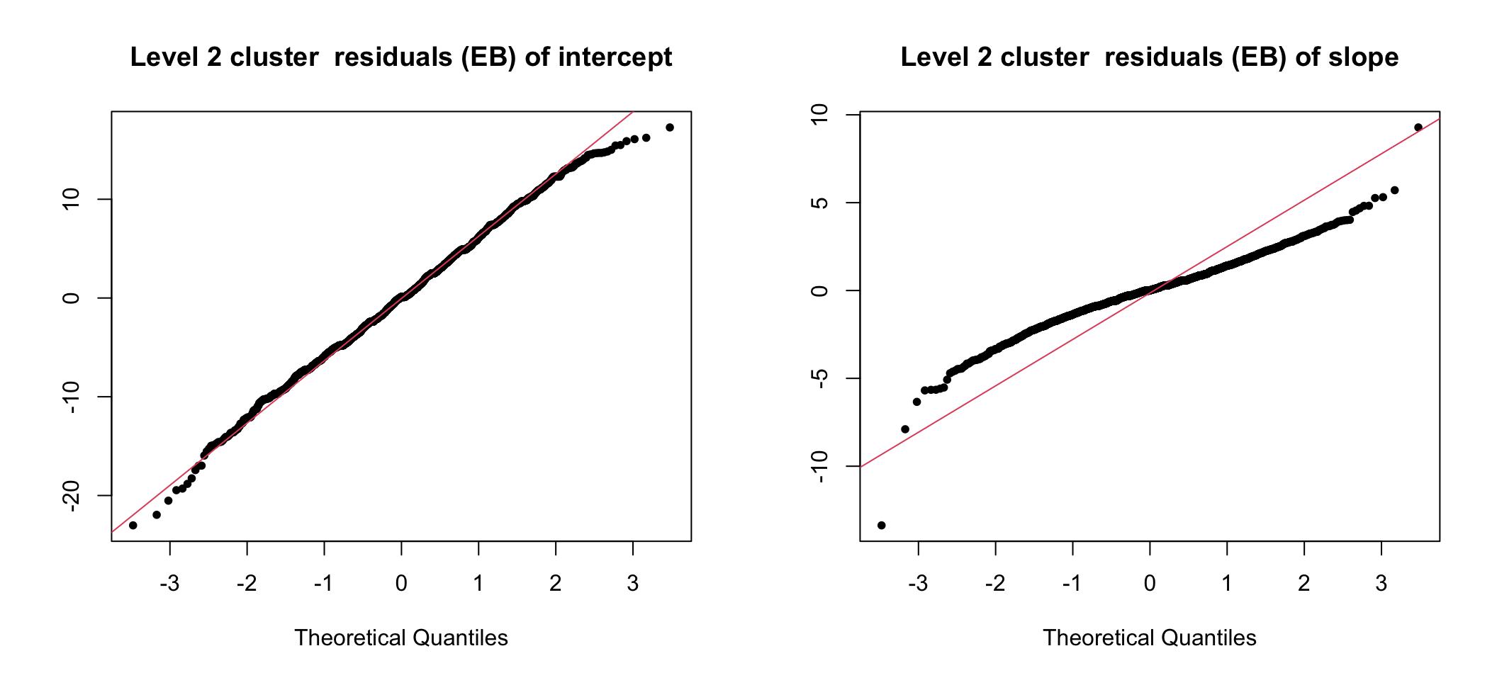
圖 76.3: UN-Standardized cluster level residuals (intercept and slope) from the random intercept and slope model
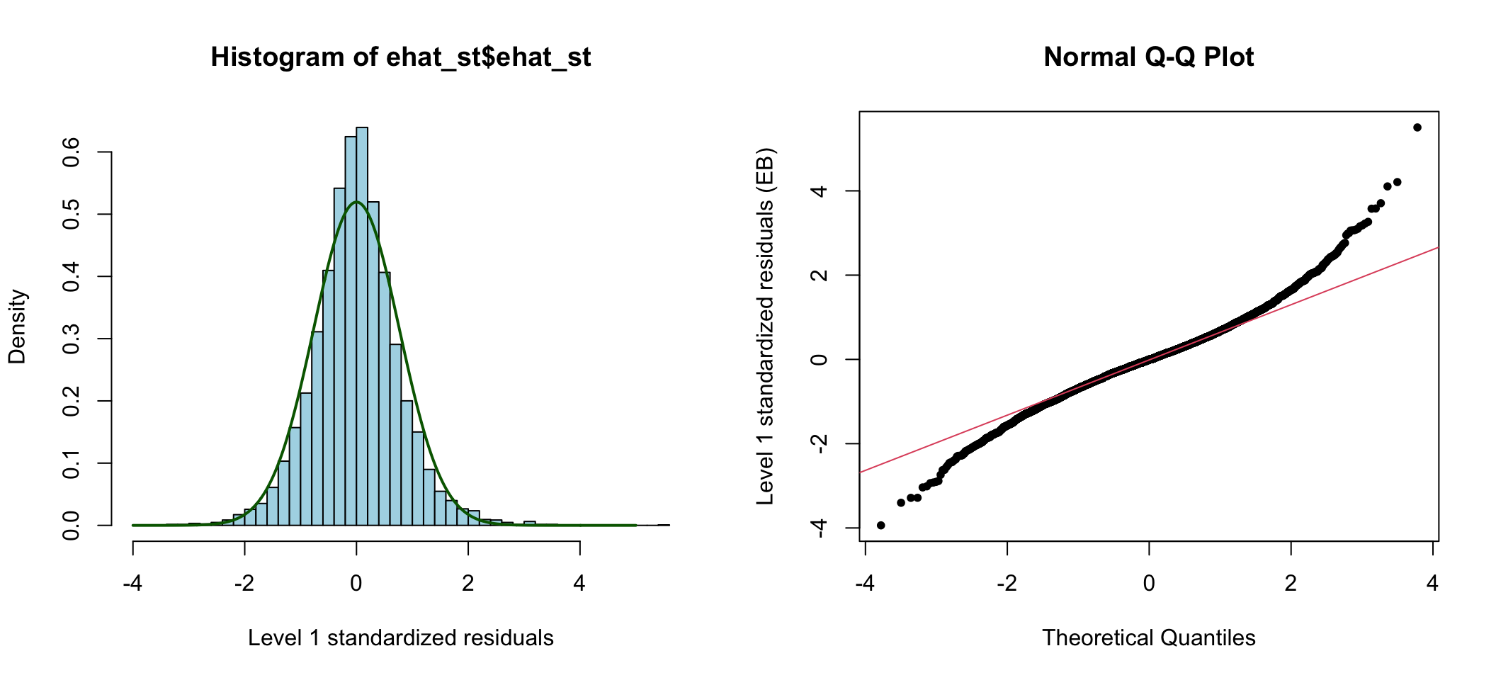
圖 76.4: Standardized elementary level residuals from the random intercept and slope model
76.2 不固定測量時刻 variable occasions
當重復收集的數據不是平衡數據時,意味着不同的人數據的收集時間點不一樣,我們就無法像前面那樣用協方差矩陣的方式來描述不同人不同時間點之間測量值可能存在的相關性,也沒有辦法給每個時間點所有人的數據做平均值作爲全部人的平均特質。
但是我們可以把不固定測量時刻的不平衡數據看作是受缺失值數據影響的平衡數據 (unbalanced data can be thought of as balanced data affected by missingness)。所以需要特別小心謹慎,因爲用線性混合效應模型擬合這樣的數據,其實是在含蓄地假設那些應該出現但是沒有出現的測量值的缺失是隨機的。
Asian growth data 實例
在本部分開頭的章節介紹過,這是一個收集了亞洲兒童在 6 周,8 個月,12 個月,和 27 個月大時的體重數據。
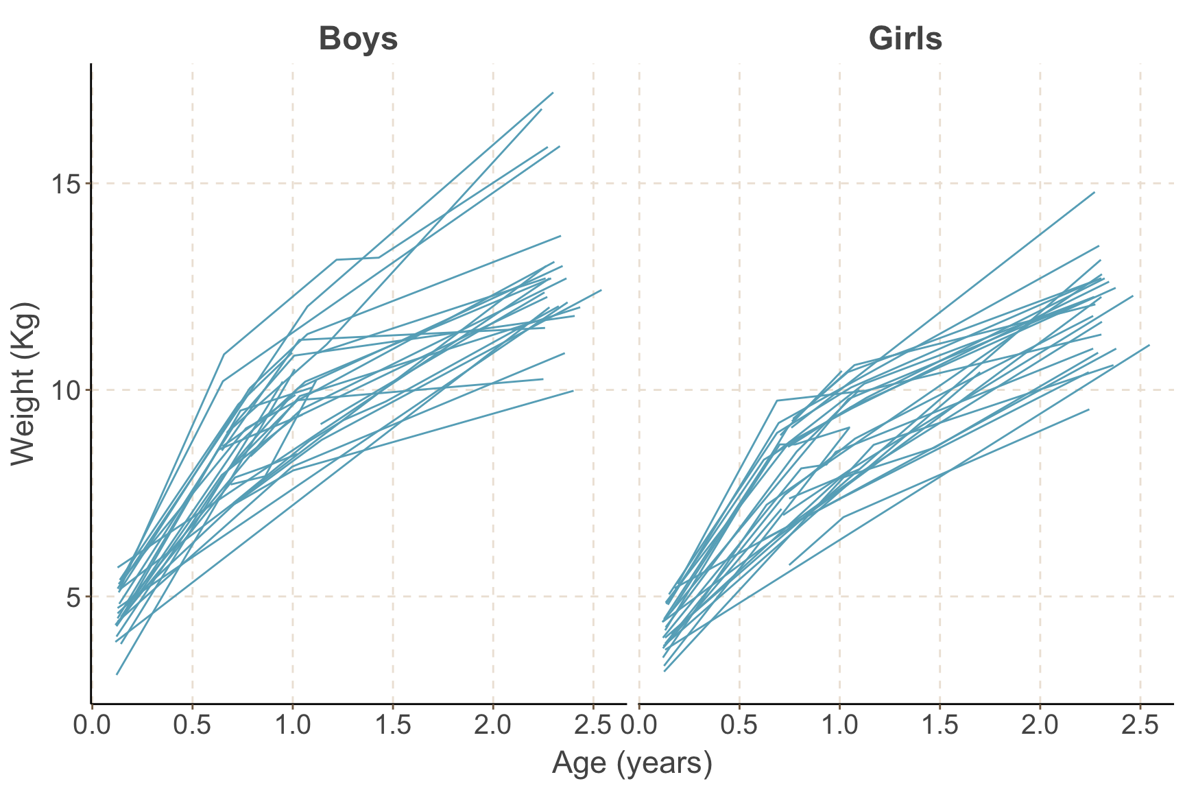
圖 76.5: Growth profiles of boys and girls in the Asian growth data
如圖 76.5 所示,觀察男孩女孩的體重隨着時間的變化,似乎暗示男孩子體重增加的速度較高,且男孩中體重增加的差異 (方差) 似乎也較女孩子的體重增加曲線來得大。另外,體重和年齡的關系並不是線性的,而且,這些數據中有缺失值。
隨機截距模型
第一個想到的合適模型應該包括一個隨機截距,一個固定效應的線性和拋物線性的年齡項,還有最後一個啞變量用以區分男孩和女孩:
\[ Y_{ij} = (\beta_0 + u_{0j}) + \beta_1t_{ij} + \beta_2 t_{ij}^2 + \beta_3 \text{girl}_j + e_{ij} \]
在 R 裏擬合這個模型:
growth <- growth %>%
  mutate(age2 = age^2)

M_growth <- lme(fixed = weight ~ age + age2 + gender, random = ~ 1 | id, data = growth, method = "REML", na.action = na.omit)
summary(M_growth)
## Linear mixed-effects model fit by REML
## Data: growth
## AIC BIC logLik
## 565.93442 585.54157 -276.96721
##
## Random effects:
## Formula: ~1 | id
## (Intercept) Residual
## StdDev: 0.85945071 0.73940625
##
## Fixed effects: weight ~ age + age2 + gender
## Value Std.Error DF t-value p-value
## (Intercept) 3.7992533 0.21210411 128 17.9122095 0.0000
## age 7.8173952 0.29051698 128 26.9085652 0.0000
## age2 -1.7054785 0.10891077 128 -15.6594104 0.0000
## genderGirls -0.7341374 0.23590992 66 -3.1119397 0.0027
## Correlation:
## (Intr) age age2
## age -0.579
## age2 0.509 -0.970
## genderGirls -0.549 -0.009 0.008
##
## Standardized Within-Group Residuals:
## Min Q1 Med Q3 Max
## -2.320321237 -0.444855166 0.024075779 0.446113187 3.991809168
##
## Number of Observations: 198
## Number of Groups: 68## 由於樣本量較小,這裏如果使用極大似然法估計 ML,結果就和 REML 估計的隨機效應的方差部分不太相同
M_growthml <- lme(fixed = weight ~ age + age2 + gender, random = ~ 1 | id, data = growth, method = "ML", na.action = na.omit)
summary(M_growthml)## Linear mixed-effects model fit by maximum likelihood
## Data: growth
## AIC BIC logLik
## 556.32603 576.05563 -272.16301
##
## Random effects:
## Formula: ~1 | id
## (Intercept) Residual
## StdDev: 0.84433851 0.73390172
##
## Fixed effects: weight ~ age + age2 + gender
## Value Std.Error DF t-value p-value
## (Intercept) 3.7997442 0.21160249 128 17.9569922 0.0000
## age 7.8161949 0.29116479 128 26.8445748 0.0000
## age2 -1.7050759 0.10915202 128 -15.6211122 0.0000
## genderGirls -0.7340920 0.23465616 66 -3.1283729 0.0026
## Correlation:
## (Intr) age age2
## age -0.582
## age2 0.511 -0.970
## genderGirls -0.548 -0.009 0.008
##
## Standardized Within-Group Residuals:
## Min Q1 Med Q3 Max
## -2.340993892 -0.446771161 0.028578899 0.450565995 4.026706851
##
## Number of Observations: 198
## Number of Groups: 68隨機截距和斜率模型
此時我們再來用相同的數據擬合混合效應模型,現在允許線性年齡的斜率有隨機變化:
M_growth_mix <- lme(fixed = weight ~ age + age2 + gender, random = ~ age | id, data = growth, method = "REML", na.action = na.omit)
summary(M_growth_mix)
## Linear mixed-effects model fit by REML
## Data: growth
## AIC BIC logLik
## 533.95003 560.0929 -258.97502
##
## Random effects:
## Formula: ~age | id
## Structure: General positive-definite, Log-Cholesky parametrization
## StdDev Corr
## (Intercept) 0.61487746 (Intr)
## age 0.51776876 0.135
## Residual 0.57411964
##
## Fixed effects: weight ~ age + age2 + gender
## Value Std.Error DF t-value p-value
## (Intercept) 3.7954977 0.168145159 128 22.572744 0.0000
## age 7.6984361 0.239853328 128 32.096433 0.0000
## age2 -1.6577339 0.088594498 128 -18.711477 0.0000
## genderGirls -0.5983844 0.199974732 66 -2.992300 0.0039
## Correlation:
## (Intr) age age2
## age -0.543
## age2 0.502 -0.929
## genderGirls -0.588 -0.008 0.007
##
## Standardized Within-Group Residuals:
## Min Q1 Med Q3 Max
## -2.041884359 -0.442600626 -0.032412585 0.419399401 2.669681983
##
## Number of Observations: 198
## Number of Groups: 68這裏可以看到隨機殘差 (residuals) 的標準差 (StdDev) 部分在後者(混合系數模型)中明顯變小了 \((0.74\rightarrow 0.54)\)。另外,第二層級殘差和第一層級殘差 (未標準化) 如圖 76.6 和 76.7:
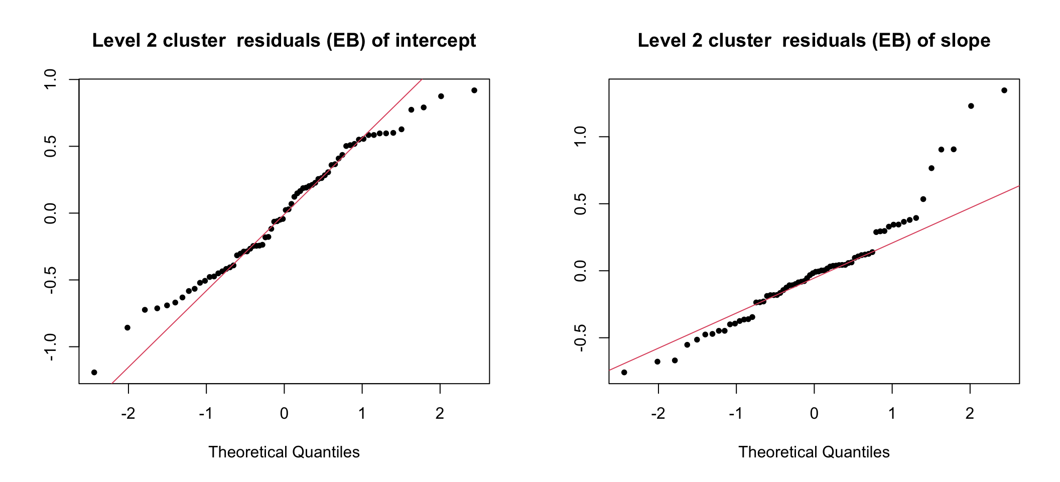
圖 76.6: UN-Standardized cluster level residuals (intercept and slope) from the random intercept and slope model
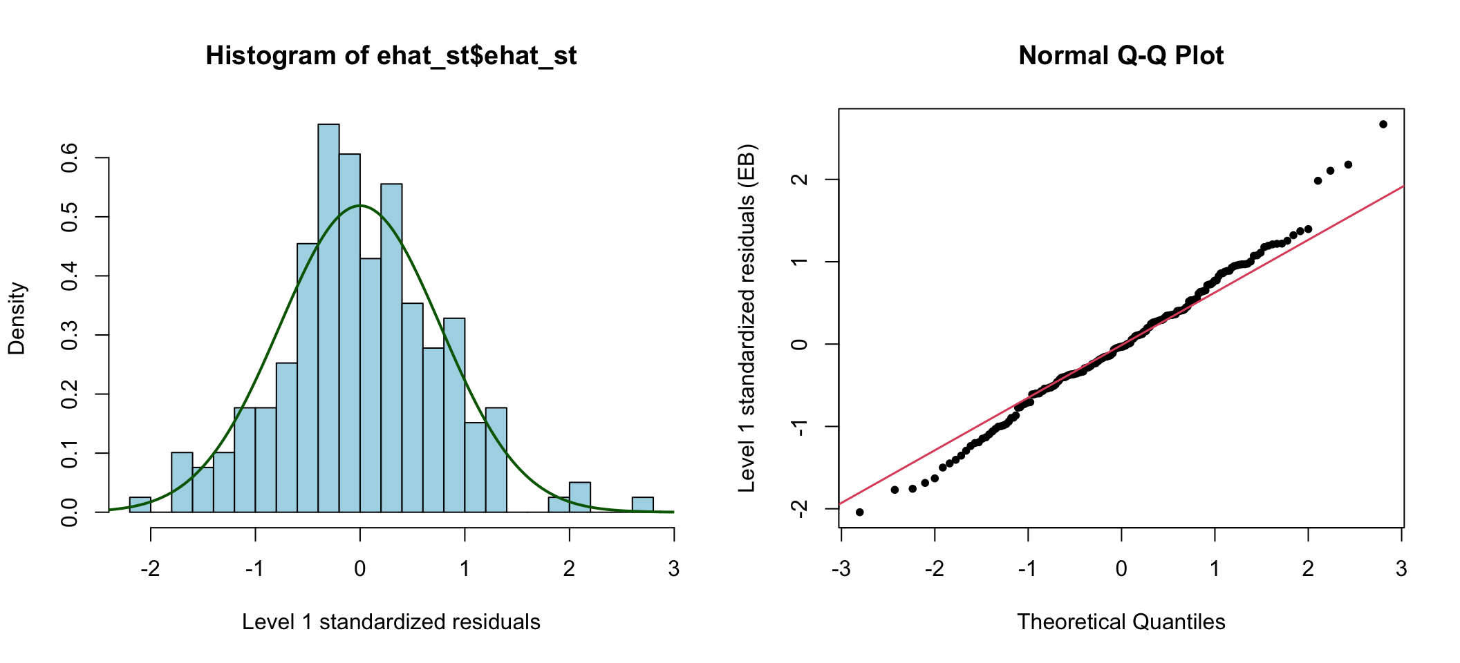
圖 76.7: Standardized elementary level residuals from the random intercept and slope model
76.3 預測軌跡 predicting trajectories
比較只有隨機截距模型,和隨機系數模型給出的擬合曲線是否有差異 如圖76.8,其實差異十分微小。可以用下面的 R 代碼:
growth$traj2 <- fitted(M_growth_mix)
growth$traj1 <- fitted(M_growth)

G <- ggplot(growth[growth$id %in% c(258,1141,3148,287),], aes(x = age, y = weight)) + geom_point(shape = 19, size = 4) +
 # geom_line(aes(y = traj1)) +
#  geom_line(aes(y = traj2), linetype = 2) +
  stat_smooth(method = "lm", aes(y = traj1), formula = y ~ x + I(x^2), se = F, linetype = 2) +
  stat_smooth(method = "lm", aes(y = traj2), formula = y ~ x + I(x^2), se = F)  +
   theme(axis.text = element_text(size = 15),
  axis.text.x = element_text(size = 15),
  axis.text.y = element_text(size = 15)) +
  theme(axis.title = element_text(size = 17), axis.text = element_text(size = 8))


G +  facet_wrap( ~ id, ncol = 2) +
  theme(strip.text = element_text(face = "bold", size = rel(1.5)))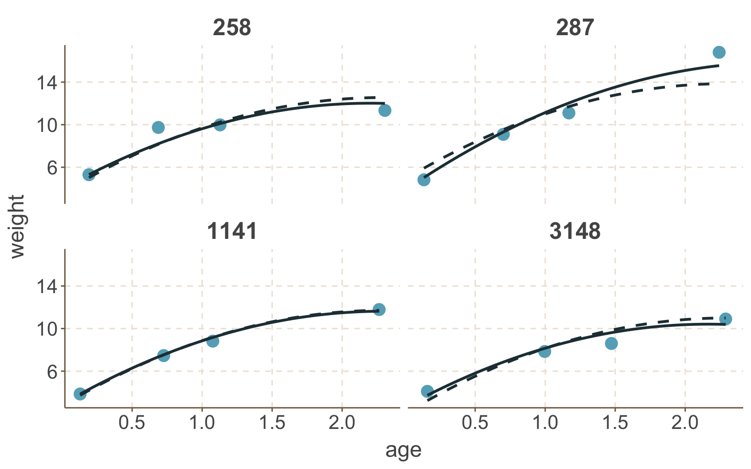
圖 76.8: Observed weight and predicted growth profiles of four babies in the Asian growth data