第 60 章 模型比較和擬合優度
我們用數據擬合廣義線性模型時其實有許多不同的目的和意義:
- 估計某些因素的暴露和因變量之間的相關程度,同時調整其餘的混雜因素;
- 確定能夠強有力的預測因變量變化的因子;
- 用於預測未來的事件或者病人的預後等等。
但是一般情況下,我們拿到數據以後不可能立刻就能構建起來一個完美無缺的模型。我們常常會擬合兩三個甚至許多個模型,探索模型和數據的擬合程度,就成爲了比較哪個模型更優於其他模型的硬指標。本章的目的是介紹 GLM 嵌套式模型之間的兩兩比較方法,其中一個模型的預測變量是另一個模型的預測變量的子集。
對手裡的數據構建一個GLM的過程,其實就是在該數據的條件下(given the data),對模型參數 \(\mathbf{\beta}\) 定義其對數似然 (log-likelihood),並尋找能給出極大值的那一系列極大似然估計 (maximum likelihood estimates, MLE) \(\mathbf{\hat\beta}\) 的過程。每次構建一個模型,我們都會獲得該模型對應的極大對數似然,它其實是極爲依賴構建它的觀察數據的,意味着每次觀察數據發生變化,你即使用了相同的模型來擬合相同的GLM獲得的極大似然都會發生變化。所以其實我們並不會十分關心這個極大似然的絕對值大小。我們關心的其實是,當對相同數據,構建了包含不同變量的模型時,極大似然的變化量。因爲這個極大似然(或者常被略稱爲對數似然 log likelihood,甚至直接只叫做似然)的變化量本身確實會反應我們思考的模型,和觀察數據之間的擬合程度。一般來說,模型中變量較少的那個 (通常叫做更加一般化的模型 more general model)獲得的似然值和變量較多的那個模型獲得的似然值相比較都會比較小,我們關心的似然值在增加了新變量之後的複雜模型後獲得的增量,是否有價值,是否真的改善了模型的擬合度 (whether the difference in log likelihoods is large enough to indicate that the less general model provides a “real” improvement in fit)。
60.1 嵌套式模型的比較 nested models
假如我們用相同的數據擬合兩個 GLM,\(\text{Model 1, Model 2}\)。其中,當限制 \(\text{Model 2}\) 中部分參數爲零之後會變成 \(\text{Model 1}\)時, 我們說 \(\text{Model 1}\) 是 \(\text{Model 2}\) 的嵌套模型。
- 例1:嵌套式模型 I
模型 1 的線性預測方程爲 \[\eta_i = \alpha + \beta_1 x_{i1}\]
模型 2 和模型 1 的因變量相同 (分佈相同),使用相同的鏈接方程 (link function) 和尺度參數 (scale parameter, \(\phi\)),但是它的線性預測方程爲 \[\eta_i = \alpha + \beta_1 x_{i1} + \beta_2 x_{i1} + \beta_3 x_{i3}\]
此時我們說模型 1 是模型 2 的嵌套模型,因爲令 \(\beta_2 = \beta_3 = 0\) 時,模型 2 就變成了 模型 1。 - 例2:嵌套式模型 II
模型 1 的線性預測方程爲 (此處默認 \(x_{i1}\) 是連續型預測變量) \[\eta_i = \alpha + \beta_1 x_{i1}\]
模型 2 的線性預測方程如果是 \[\eta_i = \alpha + \beta_1 x_{i1} + \beta_2 x^2_{i1}\]
此時我們依然認爲 模型 1 是模型 2 的嵌套模型, 因爲令 \(\beta_2 = 0\) 時,模型 2 就變成了 模型 1。
關於嵌套式模型,更加一般性的定義是這樣的:標記模型 2 的參數向量是 \(\mathbf{(\psi, \lambda)}\),其中,當我們限制了參數向量的一部分例如 \(\mathbf{\psi = 0}\),模型 2 就變成了 模型 1 的話,模型 1 就是嵌套於 模型 2 的。所以比較嵌套模型之間的擬合度,我們可以比較較爲複雜的 模型 2 相較 模型 1 多出來的複雜的預測變量參數部分 \(\mathbf{\psi}\) 是否是必要的。也就是說,比較嵌套模型哪個更優的情況下,零假設是 \(\mathbf{\psi = 0}\)。
這是典型的多變量的模型比較,需要用到子集似然比檢驗 19,log-likelihood ratio test:
\[ \begin{aligned} -2pllr(\psi = 0) & = -2\{ \ell_p(\psi=0) - \ell_p(\hat\psi) \} \stackrel{\cdot}{\sim} \chi^2_{df}\\ \text{Where } \hat\psi & \text{ denotes the MLE of } \psi \text{ in Model 2} \\ \text{With } df & = \text{ the dimension of } \mathbf{\psi} \end{aligned} \]
\(\ell_p(\psi=0)\),其實是 模型 1 的極大對數似然,記爲 \(\ell_1\)。\(\ell_p(\hat\psi)\) 其實是 模型 2 的極大對數似然,記爲 \(\ell_2\)。所以這個似然比檢驗統計量就變成了:
\[ -2pllr(\psi = 0) = -2(\ell_1-\ell_2) \]
這個統計量在零假設的條件下服從自由度爲兩個模型參數數量之差的卡方分佈。如果 \(p\) 值小於提前定義好的顯著性水平,將會提示有足夠證據證明 模型 2 比 模型 1 更好地擬合數據。
60.2 嵌套式模型比較實例
回到之前用過的瘋牛病和牲畜羣的數據 59.5。我們當時成功擬合了兩個 GLM 模型,模型 1 的預測變量只有 “飼料”,“羣”;模型 2 的預測變量在模型 1 的基礎上增加二者的交互作用項。並且我們當時發現交互作用項部分並無實際統計學意義 \(p = 0.584\)。現在用對數似然比檢驗來進行類似的假設檢驗。
先用 logLik(Model) 的方式提取兩個模型各自的對數似然,然後計算對數似然比,再去和自由度爲 1 (因爲兩個模型只差了 1 個預測變量) 的卡方分佈做比較:
Model1 <- glm(cbind(infect, cattle - infect) ~ factor(group) + dfactor, family = binomial(link = logit), data = Cattle)
Model2 <- glm(cbind(infect, cattle - infect) ~ factor(group) + dfactor + factor(group)*dfactor, family = binomial(link = logit), data = Cattle)
logLik(Model1)
## 'log Lik.' -13.12687 (df=3)## 'log Lik.' -12.973836 (df=4)LLR <- -2*(logLik(Model1) - logLik(Model2))
1-pchisq(as.numeric(LLR), df=1) # p value for the LLR test## [1] 0.58010367再和 lmtest::lrtest 的輸出結果作比較。
## Likelihood ratio test
##
## Model 1: cbind(infect, cattle - infect) ~ factor(group) + dfactor
## Model 2: cbind(infect, cattle - infect) ~ factor(group) + dfactor + factor(group) *
##     dfactor
##   #Df   LogLik Df   Chisq Pr(>Chisq)
## 1   3 -13.1269
## 2   4 -12.9738  1 0.30607     0.5801
結果跟我們手計算的結果完全吻合。AWESOME !!!
值得注意的是,此時進行的似然比檢驗結果獲得的 p 值,和模型中 Wald 檢驗結果獲得的 p 值十分接近 (0.5801 v.s. 0.584),這也充分顯示了這兩個檢驗方法其實是漸進相同的 (asymptotically equivalent)。
60.3 飽和模型,模型的偏差,擬合優度
在簡單線性迴歸中,殘差平方和提供了模型擬合數據好壞的指標 – 決定係數 \(R^2\) (Section 29.2.3),並且在 偏 F 檢驗 (Section 31.3.4) 中得到模型比較的應用。
廣義線性迴歸模型中事情雖然沒有這麼簡單,但是思想可以借鑑。先介紹飽和模型 (saturated model) 的概念,再介紹其用於模型偏差 (deviance) 比較的方法。前文中介紹過的嵌套模型之間的對數似然比檢驗,也是測量兩個模型之間偏差大小的方法。
60.3.1 飽和模型 saturated model
飽和模型 saturated model,是指一個模型中所有可能放入的參數都被放進去的時候,模型達到飽和,自由度爲零。其實就是模型中參數的數量和觀測值個數相等的情況。飽和模型的情況下,所有的擬合值和對應的觀測值相等。所以,對於給定的數據庫,飽和模型提供了所有模型中最 “完美” 的擬合值,因爲擬合值和觀測值完全一致,所以飽和模型的對數似然,比其他所有你建立的模型的對數似然都要大。但是多數情況下,飽和模型並不是合理的模型,不能用來預測也無法拿來解釋數據,因爲它本身就是數據。
60.3.2 模型偏差 deviance
令 \(L_c\) 是目前擬合模型的對數似然,\(L_s\) 是數據的飽和模型的對數似然,所以兩個模型的對數似然比是 \(\frac{L_c}{L_s}\)。那麼尺度化的模型偏差 (scaled deviance) \(S\) 被定義爲:
\[ S=-2\text{ln}(\frac{L_c}{L_s}) = -2(\ell_c - \ell_s) \]
值得注意的是,非尺度化偏差 (unscaled deviance) 被定義爲 \(\phi S\),其中的 \(\phi\) 是尺度參數,由於泊松分佈和二項分佈的尺度參數都等於 1 (\(\phi = 1\)),所以尺度化偏差和非尺度化偏差才會在數值上相等。
這裏定義的模型偏差大小,可以反應一個模型擬合數據的程度,偏差越大,該模型對數據的擬合越差。“Deviance can be interpreted as Badness of fit”.
但是,模型偏差只適用於彙總後的二項分佈數據(aggregated)。當數據是個人的二進制數據時 (inidividual binary data),模型的偏差值變得不再適用,無法用來比較模型對數據的擬合程度。 這是因爲當你的觀測值 (個人數據) 有很多時,擬合飽和模型所需要的參數個數會趨向於無窮大,這違背了子集對數似然比檢驗的條件。
60.3.3 彙總型二項分佈數據 aggregated/grouped binary data
假如,觀察數據是互相獨立的,服從二項分佈的 \(n\) 個觀測值: \(Y_i \sim Bin(n_i, \pi_i), i=1,\dots,n\)。用彙總型的數據表達方法來描述它,那麼獲得的數據就是一個個分類變量在各自組中的人數或者百分比的數據 (如下面的數據所示)。這樣的數據的飽和模型,其實允許了每個分類變量的組中百分比變化 (The saturated model for this data allows the probability of “success” to be different in each group, so that \(\tilde{\pi} = \frac{y_i}{n_i}\))。也就是每組的模型擬合後百分比,等於觀察到的百分比。
##    dose n_deaths n_subjects
## 1 49.06        6         59
## 2 52.99       13         60
## 3 56.91       18         62
## 4 60.84       28         56
## 5 64.76       52         63
## 6 68.69       53         59
## 7 72.61       60         62
## 8 76.54       59         60
那麼彙總型二項分佈數據,其飽和模型的對數似然其實就是
\[ \ell_s = \sum_{i = 1}^n\{ \log\binom{n_i}{y_i} + y_i\log(\tilde{\pi_i}) + (n_i - y_i)\log(1 - \tilde{\pi_i}) \} \]
假設此時我們給這個數據擬合一個非飽和模型,該模型告訴我們每個分類組中的預測百分比是 \(\hat\pi_i, i = 1, \dots, n\),那麼這個非飽和模型的對數似然其實是
\[ \ell_c = \sum_{i = 1}^n\{ \binom{n_i}{y_i} + y_i\log(\hat\pi_i) + (n_i - y_i)\log(1-\hat\pi_i)\} \]
那麼這個非飽和模型的模型偏差 (deviance) 就等於
\[ \begin{aligned} S & = -2(\ell_c - \ell_s) \\ & = 2\sum_{i = 1}^n\{ y_i\log(\frac{\tilde{\pi_i}}{\hat\pi_i}) + (n_i - y_i)\log(\frac{1-\tilde{\pi_i}}{1-\hat\pi_i}) \} \end{aligned} \]
從上面這個表達式不難看出,模型偏差值的大小,將會隨着模型預測值的變化而變化,如果它更加接近飽和模型的預測值 (飽和模型的預測值其實就等於觀測值),那麼模型的偏差就會比較小。如果你的彙總型數據擬合了你認爲合適的模型以後,你發現它的模型偏差值很大,那麼就意味着你的模型預測值其實和觀測值相去甚遠,模型和觀測值的擬合度應該不理想。對於彙總型數據來說,模型偏差值,其實等價於將你擬合的模型和飽和模型之間做子集對數似然比檢驗 (profile log-likelihood ratio test)。漸進來說 (asymptotically),這個子集對數似然比檢驗的結果,會服從自由度爲 \(n-p\) 的 \(\chi^2\) 分佈,其中 \(n, p\) 分別是飽和模型和你擬合的模型中被估計參數的個數。
60.4 個人數據擬合模型的優度檢驗
在上文中已經提到了,當你的數據不再是彙總型二項分佈數據,而是個人二項分佈數據 (individual binary data) 時,模型偏差 (deviance) 無法用來評價你建立的模型。這樣的數據其實比彙總型二項分佈數據更加常見,當模型中一旦需要加入一個連續型變量時,數據就只能被表達爲個人二項分佈數據。對於個人二項分佈數據模型擬合度比較,最常用的方法是 (Hosmer and Lemesbow 1980) 提出的模型擬合優度檢驗法 (goodness of fit)。該方法的主要思想是,把個人二項分佈數據模型獲得的個人預測值 (model predicted probabilities) \(\hat\pi_i\) 進行人爲的分組,把預測值數據強行變成彙總型二項分佈數據,那麼觀測值的樣本量即使增加到無窮大,也不會使得模型中組別增加到無窮大,從而可以規避
在 R 裏面,進行邏輯迴歸模型的擬合優度檢驗的自定義方程如下,參考網站:
hosmer <- function(y, fv, groups=10, table=TRUE, type=2) {
 # A simple implementation of the Hosmer-Lemeshow test
   q <- quantile(fv, seq(0,1,1/groups), type=type)
   fv.g <- cut(fv, breaks=q, include.lowest=TRUE)
   obs <- xtabs( ~ fv.g + y)
   fit <- cbind( e.0 = tapply(1-fv, fv.g, sum), e.1 = tapply(fv, fv.g, sum))
   if(table) print(cbind(obs,fit))
   chi2 <- sum((obs-fit)^2/fit)
   pval <- pchisq(chi2, groups-2, lower.tail=FALSE)
   data.frame(test="Hosmer-Lemeshow",groups=groups,chi.sq=chi2,pvalue=pval)
 }
# lbw <- read_dta("http://www.stata-press.com/data/r12/lbw.dta")
lbw <- read_dta(file = "../backupfiles/lbw.dta")
lbw$race <- factor(lbw$race)
lbw$smoke <- factor(lbw$smoke)
lbw$ht <- factor(lbw$ht)
Modelgof <- glm(low ~ age + lwt + race + smoke + ptl + ht + ui,
data = lbw, family = binomial(link = logit))
hosmer(lbw$low, fitted(Modelgof))## 0 1 e.0 e.1
## [0.0273,0.0827] 19 0 17.8222227 1.1777773
## (0.0827,0.128] 17 2 16.9739017 2.0260983
## (0.128,0.201] 13 6 15.8285445 3.1714555
## (0.201,0.243] 18 1 14.6957098 4.3042902
## (0.243,0.279] 12 7 14.1062047 4.8937953
## (0.279,0.314] 12 7 13.3601242 5.6398758
## (0.314,0.387] 13 6 12.4628053 6.5371947
## (0.387,0.483] 12 7 10.8241660 8.1758340
## (0.483,0.594] 9 10 8.6901416 10.3098584
## (0.594,0.839] 5 13 5.2361795 12.7638205## test groups chi.sq pvalue
## 1 Hosmer-Lemeshow 10 9.6506834 0.29040407## 0 1 e.0 e.1
## [0.0273,0.128] 36 2 34.796124 3.2038756
## (0.128,0.243] 31 7 30.524254 7.4757458
## (0.243,0.314] 24 14 27.466329 10.5336711
## (0.314,0.483] 25 13 23.286971 14.7130287
## (0.483,0.839] 14 23 13.926321 23.0736789## test groups chi.sq pvalue
## 1 Hosmer-Lemeshow 5 2.435921 0.4869829760.5 GLM Practical 04
60.5.1 回到之前的昆蟲數據,嘗試評價該模型的擬合優度。
- 重新讀入昆蟲數據,擬合前一個練習中擬合過的模型,使用
glm()命令。
Insect <- read.table("../backupfiles/INSECT.RAW", header =  FALSE, sep ="", col.names = c("dose", "n_deaths", "n_subjects"))
# print(Insect)
Insect <- Insect %>%
  mutate(p = n_deaths/n_subjects)

Model1 <- glm(cbind(n_deaths, n_subjects - n_deaths) ~ dose,
              family = binomial(link = logit), data = Insect)
summary(Model1); jtools::summ(Model1, digits = 6, confint = TRUE, exp = TRUE)
##
## Call:
## glm(formula = cbind(n_deaths, n_subjects - n_deaths) ~ dose,
## family = binomial(link = logit), data = Insect)
##
## Deviance Residuals:
## Min 1Q Median 3Q Max
## -1.14983 -0.22403 0.25301 0.70846 0.99107
##
## Coefficients:
## Estimate Std. Error z value Pr(>|z|)
## (Intercept) -14.086403 1.228393 -11.467 < 2.2e-16 ***
## dose 0.236593 0.020303 11.653 < 2.2e-16 ***
## ---
## Signif. codes: 0 '***' 0.001 '**' 0.01 '*' 0.05 '.' 0.1 ' ' 1
##
## (Dispersion parameter for binomial family taken to be 1)
##
## Null deviance: 268.26829 on 7 degrees of freedom
## Residual deviance: 4.61548 on 6 degrees of freedom
## AIC: 37.394
##
## Number of Fisher Scoring iterations: 4| Observations | 8 |
| Dependent variable | cbind(n_deaths, n_subjects - n_deaths) |
| Type | Generalized linear model |
| Family | binomial |
| Link | logit |
| 𝛘²(1) | 263.652801 |
| Pseudo-R² (Cragg-Uhler) | 1.000000 |
| Pseudo-R² (McFadden) | 0.887580 |
| AIC | 37.393985 |
| BIC | 37.552868 |
| exp(Est.) | 2.5% | 97.5% | z val. | p | |
|---|---|---|---|---|---|
| (Intercept) | 0.000001 | 0.000000 | 0.000008 | -11.467341 | 0.000000 |
| dose | 1.266925 | 1.217500 | 1.318357 | 11.653009 | 0.000000 |
| Standard errors: MLE |
- 根據上面模型輸出的結果,檢驗是否有證據證明該模型對數據的擬合不佳。
上面模型擬合的輸出結果中,可以找到最下面的模型偏差值的大小和相應的自由度: Residual deviance: 4.6155 on 6 degrees of freedom。如果我們要檢驗該模型中假設的前提條件之一–昆蟲死亡的對數比值 (on a log-odds scale) 和藥物濃度 (dose) 之間是線性關係(或者你也可以說,檢驗是否有證據證明該模型對數據擬合不佳),我們可以比較計算獲得的模型偏差值在自由度為 6 的卡方分布 (\(\chi^2_6\)) 中出現的概率。這裡自由度 6 是由 \(n - p = 8 - 2\) 計算獲得,其中 \(n\) 是數據中觀察值個數,\(p\) 是模型中估計的參數的個數。檢驗方法很簡單:
## [1] 0.59398469所以,檢驗的結果,P 值就是 0.594,沒有任何證據反對零假設(模型擬合數據合理)。
- 試比較兩個模型對數據的擬合效果孰優孰劣:模型1,上面的模型;模型2,加入劑量的平方 (dose2),作為新增的模型解釋變量。嵌套式模型之間的比較使用的是似然比檢驗法 (profile likelihood ratio test),試着解釋這個比較方法和 Wald 檢驗之間的區別。
Model2 <- glm(cbind(n_deaths, n_subjects - n_deaths) ~ dose + I(dose^2), family = binomial(link = logit), data = Insect)
summary(Model2)
##
## Call:
## glm(formula = cbind(n_deaths, n_subjects - n_deaths) ~ dose +
## I(dose^2), family = binomial(link = logit), data = Insect)
##
## Deviance Residuals:
## 1 2 3 4 5 6 7 8
## -0.004545 0.634377 -0.691056 -0.681962 1.223967 -0.154036 -0.029880 -0.561968
##
## Coefficients:
## Estimate Std. Error z value Pr(>|z|)
## (Intercept) -2.4881722 9.8677198 -0.2522 0.8009
## dose -0.1500054 0.3291786 -0.4557 0.6486
## I(dose^2) 0.0031871 0.0027273 1.1686 0.2426
##
## (Dispersion parameter for binomial family taken to be 1)
##
## Null deviance: 268.26829 on 7 degrees of freedom
## Residual deviance: 3.18361 on 5 degrees of freedom
## AIC: 37.9621
##
## Number of Fisher Scoring iterations: 4## Analysis of Deviance Table
##
## Model 1: cbind(n_deaths, n_subjects - n_deaths) ~ dose
## Model 2: cbind(n_deaths, n_subjects - n_deaths) ~ dose + I(dose^2)
## Resid. Df Resid. Dev Df Deviance
## 1 6 4.61548
## 2 5 3.18361 1 1.43188## [1] 0.23176444兩個模型比較的結果表明,無證據反對零假設(只用線性關係擬合數據是合理的),也就是說增加劑量的平方這一新的解釋變量並不能提升模型對數據的擬合程度。仔細觀察模型2的輸出結果中,可以發現 I(dose^2) 項的 Wald 檢驗結果是 p = 0.24,十分接近似然比檢驗的結果。因為它們兩者是漸近相同的 (asymptotically equivalent)。
60.5.2 低出生體重數據
- 讀入該數據,試分析數據中和低出生體重可能相關的變量:
## # A tibble: 6 × 11
##      id   low   age   lwt      race         smoke   ptl    ht    ui   ftv   bwt
##   <dbl> <dbl> <dbl> <dbl> <dbl+lbl>     <dbl+lbl> <dbl> <dbl> <dbl> <dbl> <dbl>
## 1    85     0    19   182 2 [black] 0 [nonsmoker]     0     0     1     0  2523
## 2    86     0    33   155 3 [other] 0 [nonsmoker]     0     0     0     3  2551
## 3    87     0    20   105 1 [white] 1 [smoker]        0     0     0     1  2557
## 4    88     0    21   108 1 [white] 1 [smoker]        0     0     1     2  2594
## 5    89     0    18   107 1 [white] 1 [smoker]        0     0     1     0  2600
## 6 91 0 21 124 3 [other] 0 [nonsmoker] 0 0 0 0 2622- 擬合一個這樣的邏輯回歸模型:結果變量使用低出生體重與否
low,解釋變量使用母親最後一次月經時體重lwt(磅)。
##
## Call:
## glm(formula = low ~ lwt, family = binomial(link = logit), data = lbw)
##
## Deviance Residuals:
##      Min        1Q    Median        3Q       Max
## -1.09482  -0.90217  -0.80197   1.36105   1.98141
##
## Coefficients:
##               Estimate Std. Error z value Pr(>|z|)
## (Intercept)  0.9957634  0.7852434  1.2681  0.20476
## lwt         -0.0140371  0.0061685 -2.2756  0.02287 *
## ---
## Signif. codes:  0 '***' 0.001 '**' 0.01 '*' 0.05 '.' 0.1 ' ' 1
##
## (Dispersion parameter for binomial family taken to be 1)
##
##     Null deviance: 234.672  on 188  degrees of freedom
## Residual deviance: 228.708  on 187  degrees of freedom
## AIC: 232.708
##
## Number of Fisher Scoring iterations: 4##
## Logistic regression predicting low
##
## OR(95%CI) P(Wald's test) P(LR-test)
## lwt (cont. var.) 0.99 (0.97,1) 0.023 0.015
##
## Log-likelihood = -114.354
## No. of observations = 189
## AIC value = 232.7081- 利用
lowess平滑曲線作圖,評價在 logit 單位上,lwt和low之間是否可以認為是線性關係。
pi <- M$fitted.values

# with(lbw, scatter.smooth(lwt, pi, pch = 20, span = 0.4, lpars =
#                  list(col = "blue", lwd = 3, lty = 1), col=rgb(0,0,0,0.004),
#                  xlab = "Mother's weight at last menstural period (lbs)",
#                  ylab = "Logit(probability) of being low birth weight",
#                  frame = FALSE))

plot(lbw$lwt, lbw$low, main="Lowess smoother plot\n of the prob of having a low brith weight baby",
     xlab = "Weight at at last menstural period (lbs)",
     ylab = "Probability")
lines(lowess(lbw$lwt, lbw$low, f = 0.7), col=2, lwd = 2)
points(lbw$lwt, pi)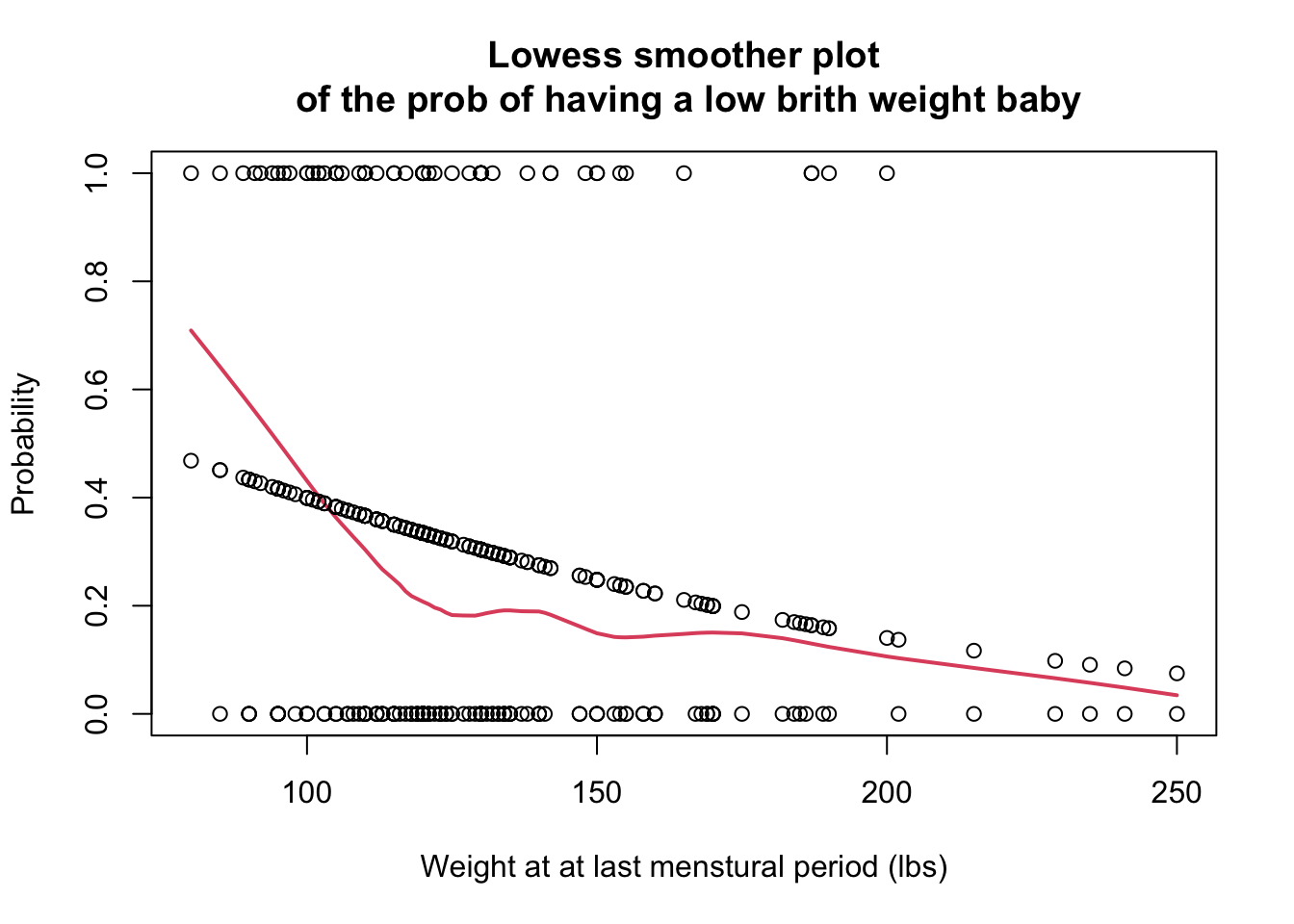
圖 60.1: The loess plot of the observed proportion with low birth weight against mother’s weight at last menstural period. Span = 0.6
Lowess 平滑曲線提示模型的擬合值(fitted.values)有一些變動,由於樣本採樣方法等原因,這是無法避免的。但是總體來說,擬合值和平滑曲線基本在同一個步調上,從該圖來看,認為母親的最後一次月經時體重和是否生下低出生體重兒的概率的 logit 之間的關係是線性的應該不是太大的問題。