第 87 章 生存數據中的回歸模型
87.1 本章概要
- 理解回歸模型對於生存數據的重要性
- 掌握如何定義不同生存分佈的回歸模型(包括指數分佈模型和 Weibull 分佈模型),並在模型中加入解釋變量。
- 理解這些不同生存分佈模型之間的異同。
- 能夠用數學表達式描述生存數據的參數模型(parametric models),包括在模型中加入解釋型變量,並考慮刪失值。
- 用極大似然法 (maximum likelihood estimation)估計生存數據參數模型中的各個參數。
- 掌握使用R來建立生存數據參數模型的方法,能看懂軟件報告的結果並作出正確的解釋。
87.2 使用參數模型分析生存數據的目的
非參數法章節 (Chapter 86) 討論的那些分析生存數據的基礎方法已經被廣泛接受並應用於比較兩組甚至是多組之間的生存函數(曲線),或風險度的異同。但是這些非參數方法的缺點也很明顯:
- 無法把連續型變量作爲暴露變量。唯一的解決方法是認爲地把連續型變量給轉換成分類型變量,然後比較落入不同區段內的對象和落入其他區段內對象之間的生存函數/風險度。
- 如果我們除了有需要比較的主要暴露還需要同時考慮混雜因子(或者互相調整),解決方法是把實驗對象人爲地分組,或者是把對象根據多個分類型暴露變量的組合進行組內的比較。這種方法最終導致劃分地越來越細的那些小組中可以用於分析的對象數據越來越少,最終不可能使分析獲得有意義的結果或解釋。
- 一般來說,我們希望同時在分析中把多個暴露變量都考慮進來,而且這些暴露變量可以同時包括連續型,二進制型,還有多分類型的變量。這樣的話使用非參數方法逐一分析變得不太有實際操作意義。
本章我們介紹用參數型回歸模型的方法來分析生存數據。這裏所說的回歸模型 (regression modelling) 其實相當類似我們學習過的簡單線性回歸模型,該模型是分析連續型結果變量和多個不同類型解釋變量;或也可以類比與廣義線性回歸中的邏輯回歸模型,即分析一個二進制結果變量和多個不同類型的解釋變量時所構建的回歸模型。之所以我們在這需要強調生存數據的參數模型 (parametric models),是由於本章節討論的生存回歸模型都假定了生存時間會服從某一個特殊形狀的分佈,這些特殊形狀的生存時間分佈本身由一個或者多個不同的參數來定義。與此形成對比的是非參數分析法中,並沒有使用任何定義生存時間分佈的參數。
87.3 生存數據的似然方程
我們來回憶一下在生存分析第一章節 (Chapter 85) 就介紹過的生存數據似然的數學表達式。
\[ L = \prod_i f(t_i)^{\delta_i}S(t_i)^{1-\delta_i} \]
- \(i = 1, \cdots, n\) 是患者的編號
- \(t_i\) 是 \(i\) 號患者的生存/刪失時間
- \(\delta_i\) 是表示 \(i\) 號患者的生存/刪失狀態的啞變量 (indicator/dummy variable)
- \(f(t_i)\) 是生存數據(死亡/事件發生患者的)的概率密度方程 probablity density function
- \(S(t_i)\) 是生存數據(生存/刪失患者的)生存概率方程 survivor function
87.4 如何加入解釋變量
讓我們先考慮簡單的情況,如果有且僅有一個二進制變量 (binary explanatory variable \(X = 0 \text{ or } 1\)) 需要加入模型中去。這個唯一的二進制解釋/暴露變量最簡單的例子就是臨牀試驗中,治療組對照組這樣的二進制變量。在這樣的情況下最簡單的比較方法就是前一章節中我們接觸過的用 log-rank 檢驗法檢驗兩條生存曲線是否有模式上的不同(定性檢驗),但是我們也知道這樣的檢驗方法並不能定量地說明當兩組之間存在生存曲線的差異時,這個差異具體有多大。
其他的二進制暴露變量的例子:
- 觀察型職業隊列研究中的暴露變量,如是否存在職業上的輻射暴露 (occupational exposure to radiation)
- 觀察型人羣隊列研究中的暴露變量,如是否吸菸 (smoker or non-smoker)
對於一個簡單的二進制暴露變量,我們認爲其中一組 \((X=1)\) 患者在時間點 \(t\) 時的風險度 (hazard) \(h_1(t)\) 和另一個被看作是對照的基準組 (baseline group \(X=0\)) 的風險度 \(h_0(t)\) 之間的關系是成比例的,即可以用乘法表達式來說明兩組之間的風險度的關係:
\[ h_1(t) = \psi h_0 (t) \]
那麼這裏的 \(\psi\) 就是我們關心的參數,需要通過獲得的數據來估計。注意這裏兩組患者的風險度,等式左右兩邊都必須是大於零的,因此 \(\psi\) 的取值要被限制在 \(>0\) 範圍。所以,我們常常直接利用指數函數的特性把它改寫成:
\[ h_1(t) = e^\beta h_0(t) \]
這樣一來,參數 \(\beta\) 就沒有了取值(是正還是負)的限制。這就是大名鼎鼎的比例風險度模型 (proportional hazard model)。\(e^\beta\) 就是風險度比 (Hazard ratio):
\[ \frac{h_1(t)}{h_0(t)} = e^\beta \]
\(\beta\) 就是對數風險度比 (log-hazard ratio),這個風險度比,不隨着時間推進而變化。所以在這種類型的生存分析的參數模型中,前提條件–比例風險度 (proportional hazard assumption),是必須被滿足的假設,且無論追蹤時間有多久,我們都默認這個(對數)風險度比是保持不變的。假如有任何證據提示你治療組對照組之間的療效差 (treatment effect) 會隨着時間發生變化的話,這個比例風險度的前提條件就被違反了。
87.5 指數模型 exponential model
我們再回頭看之前介紹過的指數模型,它是最簡單的生存時間分析參數模型。它的幾個特徵方程再次描述如下
風險度方程 hazard function:
\[ h(t) = \lim_{\delta\rightarrow0}\frac{1}{\delta}\text{Pr}(t\leqslant T <t + \delta | T>t) = \lambda \]
生存概率方程 survivor function:
\[ S(t) = \text{Pr}(T>t) = \exp\{-\lambda t\} \]
概率密度方程 probability density function:
\[ f(t) = \lambda \exp\{ - \lambda t\} \]
記得當生存數據服從指數分布時,風險度 (hazard) 本身 (而不僅僅是比例) 保持不變。這也意味着事件發生的率 (rate of the event) 不隨時間發生變化 (constant over time)。
在指數分布模型下加入解釋變量:
\[ \left\{ \begin{array}{ll} h(t;0) = \lambda & X=0 \\ h(t;1) = \lambda e^\beta & X=1 \end{array} \right. \]
這個聯立方程等價於:
\[ h(t;x) = \lambda e^{\beta x} \]
類似地,風險度方程已知了的話,概率密度方程和生存方程可以寫作:
\[ f(t;x) = \lambda e^{\beta x} \exp({-\lambda t^{\beta x}}); \\ S(t;x) = \exp(-\lambda t^{\beta x}) \]
此時的似然方程就是
\[ L = \prod_{i = 1}^n\{\lambda e^{\beta x} \exp({-\lambda t^{\beta x}}) \}^{\delta_i}\{ \exp(-\lambda t^{\beta x})\}^{1-\delta_i} \]
此時,似然方程中兩個參數 \(\lambda, \beta\) 可以利用極大似然函數的方法分別對其中一個求導數獲得 MLE,然後用 Fisher information matrix 計算各自的標準誤,從而計算 95% 信賴區間。這裏的 \(\beta\) 回歸系數,可以做是否爲零 (等價於比較 \(e^\beta = 1\)) 的 Wald 檢驗:
\[ \frac{\hat\beta}{SE(\hat\beta)} \sim N(0,1) \]
Example 87.1 推導\(\lambda,\beta\)的MLE:
\[ \begin{aligned} L & = \prod_{i = 1}^n\{\lambda e^{\beta x} \exp({-\lambda t^{\beta x}}) \}^{\delta_i}\{ \exp(-\lambda t^{\beta x})\}^{1-\delta_i} \\ & = \prod_{i = 1}^n\{\lambda e^{\beta x}\}^{\delta_i}\exp(-\lambda t^{\beta x}) \\ \Rightarrow \ell & = \log(\lambda)\sum_{i=1}^n \delta_i + \beta \sum_{i = 1}^n(x_i\delta_i) - \lambda\sum_{i = 1}^n t_ie^{\beta x_i} \\ \text{Let} & \sum_{i = 1}^n = n_1 \text{(numer of events)}; \\ &\sum_{i=1}^n(x_i\delta_i) = n_{11} \text{(number of events in } x=1); \\ &\sum_{x_i=1}^n t_i = T_1 \text{(sum of survival/censors T in } x=1);\\ &\sum_{x_i=0}^n t_i = T_0 \text{(sum of survival/censors T in } x=0);\\ \Rightarrow \ell & =n_1 \log(\lambda) + n_{11}\beta - \lambda(T_0 + T_1e^\beta) \end{aligned} \]
接下來求 MLE 就等同於解下面的聯立方程組:
\[ \left\{\begin{array}{l} \frac{\text{d}\ell}{\text{d}\lambda} = \frac{n_1}{\lambda} - (T_0 +T_1e^\beta) =0 \\ \frac{\text{d}\ell}{\text{d}\beta} = n_{11} = T_1\lambda e^\beta = 0 \end{array} \right. \\ \hat\lambda = \frac{n_1 - n_{11}}{T_0} \\ \hat\beta = \log\frac{T_0n_{11}}{T_1(n_1 - n_{11})} \]
Example 87.2 白血病患者病情緩解數據:我們對該數據使用指數模型來分析,使用Stata 或者 R就可以獲取下面表格中的分析結果。
| Parameter | Estimate | Standard error | 95% confidence interval | p-value |
|---|---|---|---|---|
| \(\lambda\) | 0.12 | 0.03 | (0.08, 0.18) | \(<\) 0.001 |
| \(\beta\) | -1.53 | 0.40 | (-2.31, -0.75) | \(<\) 0.001 |
| \(\exp \beta\) | 0.22 | 0.09 | (0.10, 0.48) | \(<\) 0.001 |
可以看到指數模型給出的風險度比的估計是 Hazard ratio = 0.22,意味着治療組白血病患者從治療開始到症狀緩解的風險率 (hazard rate) 要低於對照組很多。而且這個風險度比明顯地在統計學上不同於 1(表示兩組之間患者無風險度差異)。改分析結果提供了極強的證據來證明:治療組患者獲得的治療藥物可能對患者的緩解沒有好處反而還有害,因此導致治療組患者的緩解,比起對照組慢很多。我們可以把模型估計的兩個暴露組的患者的生存函數曲線繪製如下圖 (87.1)
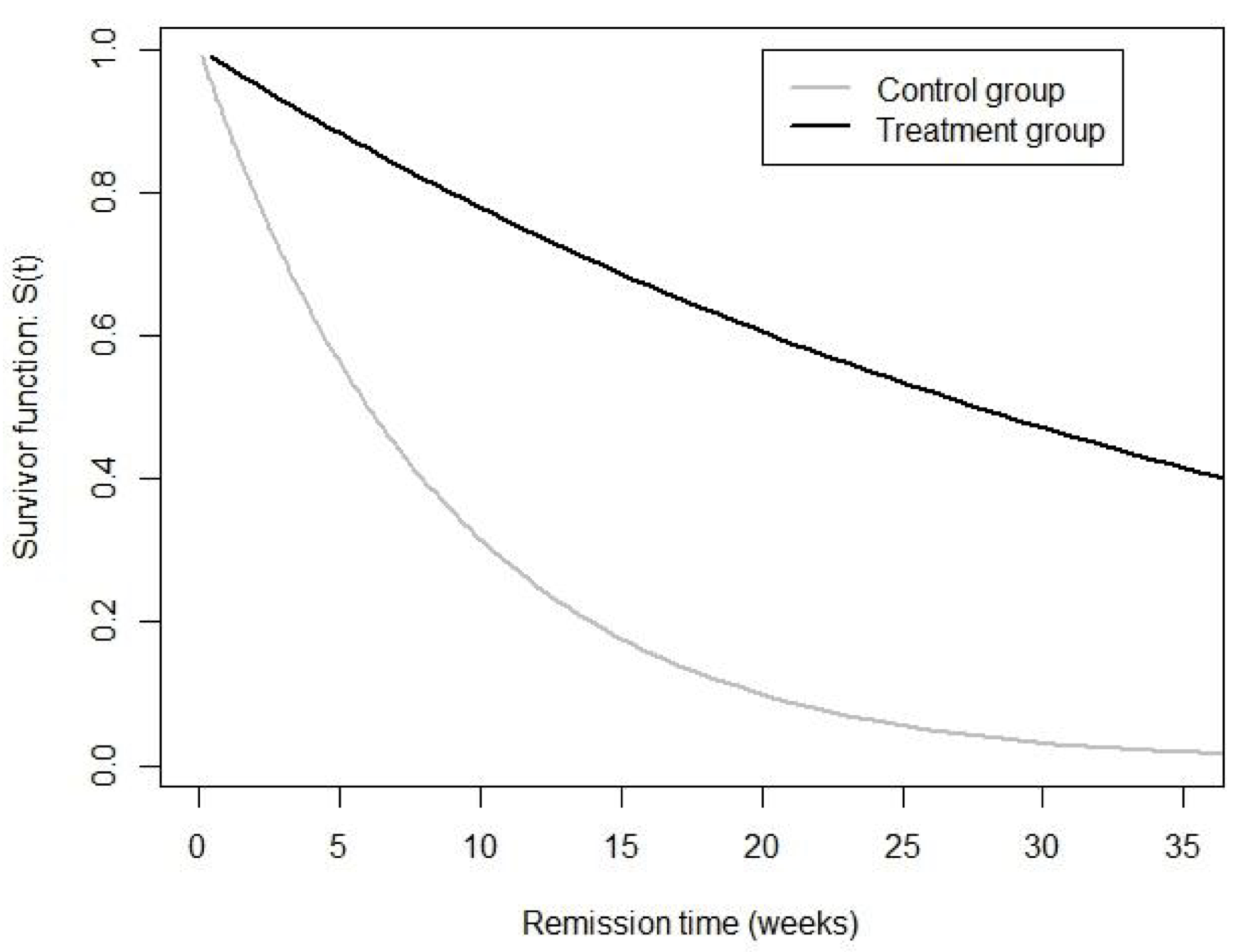
圖 87.1: Leukaemia patient data: estimated survivor curves under an exponential model.
實際在R裏的計算過程:
gehan <- read.table("https://data.princeton.edu/wws509/datasets/gehan.dat")
names(gehan)[3] <- "remission"


exp.model <- survreg(Surv(time = weeks, event = remission) ~ group,
                     dist = "exponential", data = gehan)
summary(exp.model)
##
## Call:
## survreg(formula = Surv(time = weeks, event = remission) ~ group,
## data = gehan, dist = "exponential")
## Value Std. Error z p
## (Intercept) 2.1595 0.2182 9.896 < 2e-16
## grouptreated 1.5266 0.3984 3.832 0.000127
##
## Scale fixed at 1
##
## Exponential distribution
## Loglik(model)= -108.5 Loglik(intercept only)= -116.8
## Chisq= 16.49 on 1 degrees of freedom, p= 0.000049
## Number of Newton-Raphson Iterations: 4
## n= 42- 風險度比的計算方法是: exp(-1.527) \(\approx\) 0.22
- 風險度比的95%信賴區間計算方法是:
- exp(-1.527 - 1.96*0.398) \(\approx\) 0.0995
- exp(-1.527 + 1.96*0.398) \(\approx\) 0.4738
- 基線風險的計算方法是: exp(-2.159) \(\approx\) 0.12
對比一下 Stata 的模型和輸出結果,觀察其差異
------------------------------------------------------------------------------
  _t | Haz. Ratio   Std. Err.       z P>|z|     [95% Conf. Interval]
------------------------------------------------------------------------------
group| .2172702     .0865625    -3.83 0.000     .0995115    .4743806
_cons| .1153846     .025179     -9.90 0.000     .0752316    .1769682
------------------------------------------------------------------------------
87.6 Weibull 分布
指數分布的模型只能用於”不隨時間改變(恆定不變)的風險率(hazard rate)“的情況。Weibull 分布放鬆了這個假設前提,不再要求恆定不變的風險率,但是它本身的假設(前提條件)則是風險率隨時間的變化是單調的 (遞增或者遞減,二者只能選一)。且 Weibull 分布其實是指數分布的一般化形式,或者說指數分布是 Weibull 分布的特殊形式。
Weibull 分布的風險度方程:
\[ h(t) = \kappa \lambda t^{\kappa - 1} \]
生存概率方程
\[ S(t;x) = \exp\{ -\lambda t^\kappa \} \]
概率密度方程
\[ f(t) = \kappa \lambda t^{\kappa - 1} \exp\{ -\lambda t^\kappa \} \]
那麼加入了一個二分類解釋變量 \(x\) 的 Weibull 比例風險度方程就是:
\[ h(t;x) = \kappa \lambda t^{\kappa - 1}e^{\beta x} \]
其生存概率方程就是:
\[ S(t;x) = \exp\{ -\lambda t^\kappa e^{\beta x}\} \]
概率密度方程是二者的乘積,那麼所有的生存數據的似然方程就是:
\[ L = \prod_{i=1}^n \{\kappa \lambda t^{\kappa - 1}e^{\beta x}\exp\{ -\lambda t^\kappa e^{\beta x}\} \}^{\delta_i}\{ \exp\{ -\lambda t^\kappa e^{\beta x}\}\}^{1-\delta_i} \]
但是,比較悲劇的是,在 Weibull 分布的生存模型中,沒有辦法簡單的獲得參數 \(\kappa, \lambda. \beta\) 的MLE。只能使用迭代法 (iterative numerical methods are required)。
Example 87.3 白血病患者病情緩解數據:我們對該數據使用Weibull模型來分析,使用Stata 或者 R就可以獲取下面表格中的分析結果。
| Parameter | Estimate | Standard error | 95% confidence interval | p-value |
|---|---|---|---|---|
| \(\lambda\) | 0.05 | 0.03 | (0.02, 0.14) | <0.001 |
| \(\kappa\) | 1.37 | - | (1.02, 1.82) | 0.034 |
| \(\beta\) | -1.73 | 0.41 | (-2.54, -0.92) | <0.001 |
| \(\exp \beta\) | 0.18 | 0.07 | (0.08, 0.40) | <0.001 |
可以發現當我們使用 Weibull 模型來跑相同的白血病患者數據時,風險度比估計值是 0.18。(與之相對比,在使用簡單的指數分佈模型時,風險度比的估計值是 0.22)
同樣地,我們可以繪製相似的模型生存曲線圖 (87.2)
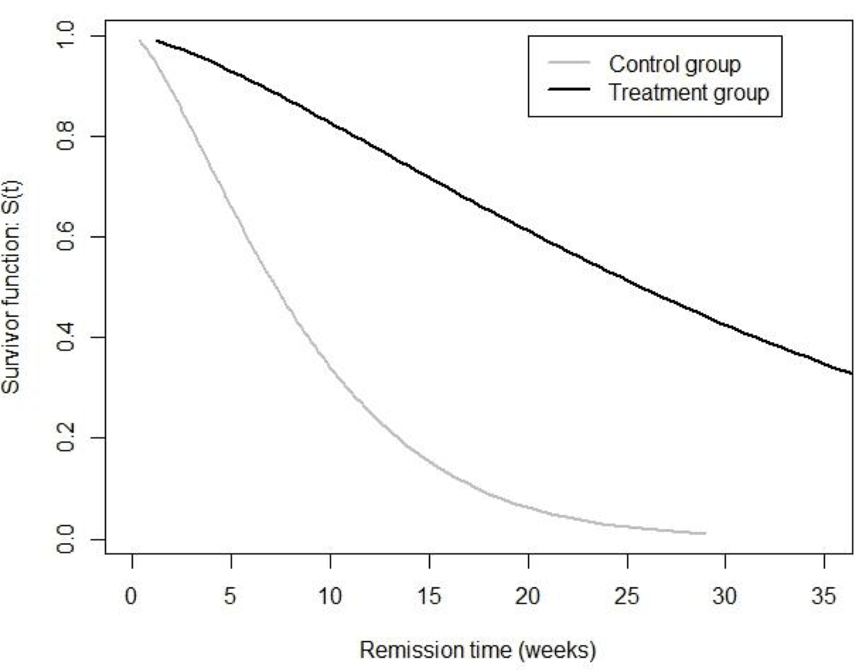
圖 87.2: Leukaemia patient data: estimated survivor curves under a Weibull model.
實際在R裏的計算過程:
weibull.model <- survreg(Surv(time = weeks, event = remission) ~ group,
                     dist = "weibull", data = gehan)
summary(weibull.model)
##
## Call:
## survreg(formula = Surv(time = weeks, event = remission) ~ group,
## data = gehan, dist = "weibull")
## Value Std. Error z p
## (Intercept) 2.2484 0.1660 13.547 < 2e-16
## grouptreated 1.2673 0.3106 4.080 0.0000451
## Log(scale) -0.3117 0.1473 -2.116 0.0343
##
## Scale= 0.7322
##
## Weibull distribution
## Loglik(model)= -106.6 Loglik(intercept only)= -116.4
## Chisq= 19.65 on 1 degrees of freedom, p= 9.3e-06
## Number of Newton-Raphson Iterations: 5
## n= 42- 風險度比的計算方法是 exp(-1.267 * exp(0.312)) \(\approx\) 0.18;
- 風險度比的95%信賴區間的計算方法是:
- exp((-1.267 - 1.96 \(\times\) 0.311) \(\times\) exp(0.312)) \(\approx\) 0.08
- exp((-1.267 + 1.96 \(\times\) 0.311) \(\times\) exp(0.312)) \(\approx\) 0.40
- 基線風險度的計算方法是 exp(- 2.248 \(\times\) exp(0.312)) \(\approx\) 0.05
實際在Stata的計算過程是:
streg group, distribution(weibull)
------------------------------------------------------------------------------
_t | Haz. Ratio Std. Err. z P>|z| [95% Conf. Interval]
-------------+----------------------------------------------------------------
group| .1771299 .0731691 -4.19 0.000 .0788272 .3980227
_cons| .0463885 .025888 -5.50 0.000 .0155375 .138497
/ln_p| .3117092 .1472919 2.12 0.034 .0230224 .600396
p | 1.365757 .201165 1.02329 1.82284
1/p | .7321944 .1078463 .5485944 .9772406
-------------+----------------------------------------------------------------87.7 Weibull 和 指數模型的比較
至此,我們可以看出,同樣的生存數據我們可以選擇使用指數模型也可以使用 Weibull 模型。問題是,哪個模型會更優於另一個?簡單說有兩種方法可以幫助你作出選擇。
- 使用繪圖輔助
- 使用統計檢驗比較
87.7.1 繪圖法
使用非參數方法獲得的圖形,有時會有助於(視覺上的方法,非正式但有助於)判斷哪種參數模型更加合適你手頭的數據。這裏用一個二進制暴露變量來做解釋。
在指數分布模型中,累積風險度 cumulative hazard 是和追蹤時間呈正比的:
\[ H(t;x) = -\log S(t;x) = \lambda t e^{\beta x} \]
在 Weibull 分布模型中,累積風險度 cumulative hazard,取了對數以後:
\[ \log H(t;x) = \log\{ -\log S(t;x) \} = \log \lambda + \kappa \log t + \beta x \]
所以,累積風險度如果取了對數,那麼這個值和時間的對數 \(\log t\) 是呈線性關系的,且當這個直線的坡度爲 1 (和橫軸呈現45度角) 的話 \(\kappa = 1\),就說明數據符合指數模型。如果,\(x\) 只是一個二分類解釋變量的話,你會看到對數累積風險度和對數時間呈現爲兩條平行線。
87.7.2 統計檢驗法
很簡單, Wald test:
\[ \frac{\log \hat\kappa}{SE(\log \hat\kappa)} \sim N(0,1) \]
當然你也可以使用似然比檢驗 likelihood ratio test,因爲指數分布模型是 Weibull 分布模型在 \(\kappa = 1\) 時的特殊形態,二者擬合的統計模型也會是嵌套式模型:
\[ -2(\ell_{\text{exponential}} - \ell_{\text{Weibull}}) \sim \chi_1^2 \]
服從的卡方分布的自由度是兩個模型的參數數量的差。似然比檢驗通常會比簡單比較 \(\kappa = 1\) 更值得實施因爲它通常會相對 wald 檢驗提供更加值得信任的檢驗,所以多數人也比較傾向於使用似然比檢驗法比較符合嵌套結構的參數模型。
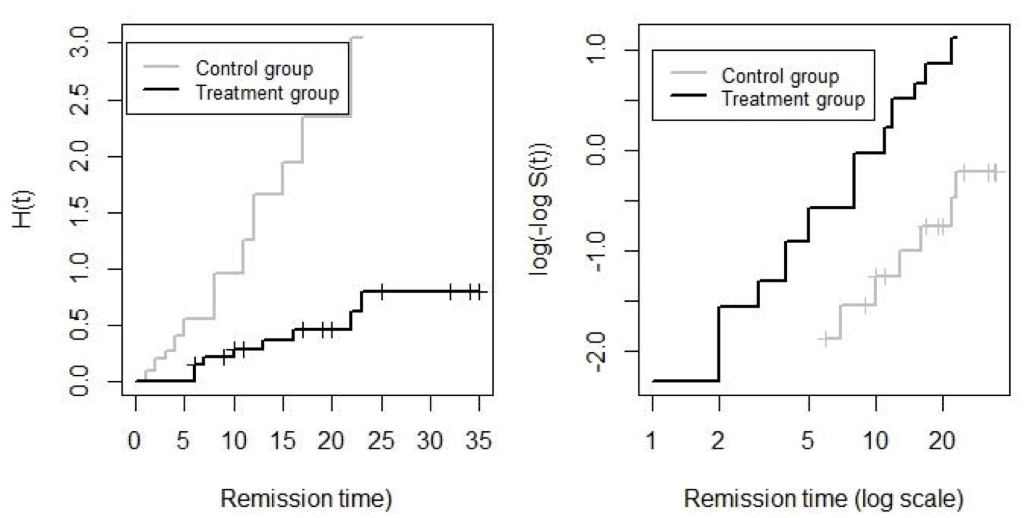
圖 87.3: Leukaemia patient data: Kaplan-Meier plots of the cumulative hazard (left) and the log cumulative hazard (right) in treatment and controls groups.
##
## Call:
## survreg(formula = Surv(time = weeks, event = remission) ~ group,
##     data = gehan, dist = "weibull")
##                Value Std. Error      z         p
## (Intercept)   2.2484     0.1660 13.547   < 2e-16
## grouptreated  1.2673     0.3106  4.080 0.0000451
## Log(scale)   -0.3117     0.1473 -2.116    0.0343
##
## Scale= 0.7322
##
## Weibull distribution
## Loglik(model)= -106.6   Loglik(intercept only)= -116.4
##  Chisq= 19.65 on 1 degrees of freedom, p= 9.3e-06
## Number of Newton-Raphson Iterations: 5
## n= 42## Likelihood ratio test
##
## Model 1: Surv(time = weeks, event = remission) ~ group
## Model 2: Surv(time = weeks, event = remission) ~ group
## #Df LogLik Df Chisq Pr(>Chisq)
## 1 3 -106.579
## 2 2 -108.524 -1 3.88912 0.0486 *
## ---
## Signif. codes: 0 '***' 0.001 '**' 0.01 '*' 0.05 '.' 0.1 ' ' 187.8 拓展解釋變量(類型與個數)的參數模型
當然可以在生存分析參數模型中加入多於一個變量,而且可以是分類型,連續型變量 \(\mathbf{X} = (X_1, X_2, \dots, X_p)^T\) :
\[ h(t;x) = h_0 (t)e^{\beta^Tx} \]
- \(h_0(t)\) 是基線組的風險度 (baseline hazard);
- \(\mathbf{\beta} = (\beta_1, \beta_2, \cdots, \beta_p)^T\) 是一組解釋變量的回歸系數;
- \(\beta_k\) 是當保持所有其他變量不變時,解釋變量 \(X_k\) 在增加/減少一個單位對應的對數風險度比 (log-hazard ratio)。
87.8.1 當變量是連續型時
對於一個連續型暴露變量 \(X\) 來說,每增加1個單位,其效果其實就是風險度乘以 \(\exp^\beta\)。所以,比較一個 \(X = 1\) 的實驗對象和一個 \(X = 0\) 的實驗對象的風險度之比:
\[ \frac{h(t : 1)}{h(t: 0)} = \frac{h_0(t) e^\beta}{h_0(t)} = e^\beta \]
如果說舉例年齡作爲唯一的暴露變量的話,73歲的人和72歲的人相比,他們之間的風險度比是:
\[ \frac{h(t : 73)}{h(t: 72)} = \frac{h_0(t) e^{73\beta}}{h_0(t) e^{72\beta}} = e^\beta \]
所以,對於一個連續型變量 \(X\) 來說,\(\beta\) 是 \(X\) 每增加一個單位時的風險度比的對數 (the log hazard ratio associated with 1 unit increase in \(X\))。
87.8.2 (多於兩種類型的)分類型變量
如果是一個多餘兩種分類(\(K + 1\))類型的變量,我們定義一系列的 \(K\) 個啞變量 (dummy variable),或者叫做指示型變量 (indicator variables)
\[ X_k = \left\{ \begin{array}{ll} 1 & \text{ if in category } k \\ 0 & \text{ otherwise } \end{array} \right. \]
那麼此時第 \(k\) 個分組的風險度是
\[ h_0(t)e^{\beta_k}, (k = 0, 1, \dots, K) \]
其中基線風險度 \(h_0(t)\) 其實是分類在第一個類別(基準組類別 \(X_0 = 1, \beta_0 = 0\))中的實驗對象的風險度。所以,\(e^{\beta_k}\) 就是比較第 \(k\) 組分類和第一個類別的實驗對象的風險度比 (the hazard ratio which compares individuals in category \(k\) with individuals in category 0)。這樣一個模型同時可以改寫成:
\[ h(t; x) = h_0(t)\exp(\beta_1x_1 + \beta_2 x_2 + \cdots + \beta_K x_K) \]
其中 \(x_k\) 是實驗對象是否屬於第 \(k\) 組分類的指示型變量。
87.9 Practical Survival 03
whitehall <- read_dta("../backupfiles/whitehall.dta")
whitehall <- whitehall %>%
                mutate(timein = as.numeric(timein),
                       timeout = as.numeric(timeout),
                       timebth = as.numeric(timebth)) %>%
                mutate(time = (timeout - timein)/365.25)

with(whitehall, tabpct(grade, chd, graph = FALSE))
##
## Original table
## chd
## grade 0 1 Total
## 1 1104 90 1194
## 2 419 64 483
## Total 1523 154 1677
##
## Row percent
## chd
## grade 0 1 Total
## 1 1104 90 1194
## (92.5) (7.5) (100)
## 2 419 64 483
## (86.7) (13.3) (100)
##
## Column percent
## chd
## grade 0 % 1 %
## 1 1104 (72.5) 90 (58.4)
## 2 419 (27.5) 64 (41.6)
## Total 1523 (100) 154 (100)#### median time
Median_t <- ddply(whitehall,c("grade","chd"),summarise,Median=median(time))
Median_t## grade chd Median
## 1 1 0 18.1779175
## 2 1 1 11.9110102
## 3 2 0 17.8726806
## 4 2 1 8.7679441whl.km <- survfit(Surv(time = time, event = chd) ~ as.factor(grade), data = whitehall)
plot(whl.km, conf.int = T, col = c("blue", "red"), mark.time = F, xlab = "Time", ylab = "Survivor function", ylim = c(0.8, 1))
legend(1, 0.85, c("Grade 1", "Grade 2"), col = c("blue", "red"), lty = 1)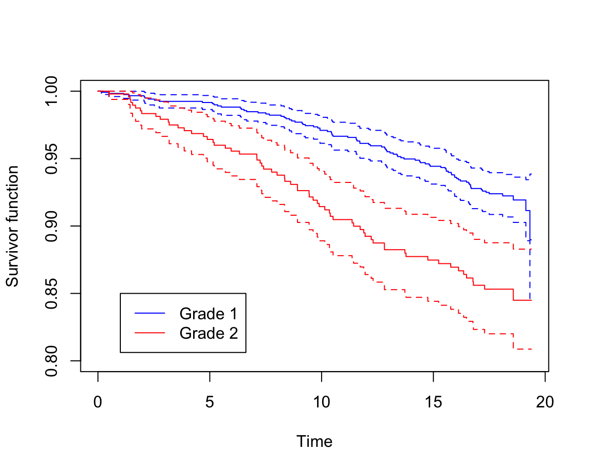
圖 87.4: Rplots of the Kaplan-Meier survivor functions
“Grade 1” 患者的生存概率明顯好於 “Grade 2”。而且,95% 信賴區間沒有重疊,提示這兩組之間的生存概率曲線應該有統計學上的顯著不同。
# How many individuals survived 5, 10, 15 years of follow-up in each job grade?
summary(whl.km, times = c(5, 10, 15))
## Call: survfit(formula = Surv(time = time, event = chd) ~ as.factor(grade),
## data = whitehall)
##
## as.factor(grade)=1
## time n.risk n.event survival std.err lower 95% CI upper 95% CI
## 5 1169 10 0.9916 0.002648 0.9864 0.9968
## 10 1114 24 0.9709 0.004913 0.9613 0.9806
## 15 1045 30 0.9443 0.006772 0.9311 0.9577
##
## as.factor(grade)=2
## time n.risk n.event survival std.err lower 95% CI upper 95% CI
## 5 445 17 0.9642 0.008521 0.9477 0.9811
## 10 383 22 0.9144 0.013135 0.8890 0.9405
## 15 334 16 0.8747 0.015876 0.8442 0.9064# Log rank test to compare the estimated survivor functions in the two job grades
survdiff(Surv(time=time, event = chd) ~ as.factor(grade), data = whitehall)## Call:
## survdiff(formula = Surv(time = time, event = chd) ~ as.factor(grade),
## data = whitehall)
##
## N Observed Expected (O-E)^2/E (O-E)^2/V
## as.factor(grade)=1 1194 90 114.19 5.123 19.85
## as.factor(grade)=2 483 64 39.81 14.692 19.85
##
## Chisq= 19.8 on 1 degrees of freedom, p= 8.4e-06# Fit an exponential model
whl.exp <- survreg(Surv(time, chd) ~ as.factor(grade), dist = "exponential", data = whitehall)
summary(whl.exp)##
## Call:
## survreg(formula = Surv(time, chd) ~ as.factor(grade), data = whitehall,
## dist = "exponential")
## Value Std. Error z p
## (Intercept) 5.4205 0.1054 51.424 < 2e-16
## as.factor(grade)2 -0.6885 0.1635 -4.211 0.0000255
##
## Scale fixed at 1
##
## Exponential distribution
## Loglik(model)= -944.7 Loglik(intercept only)= -953.1
## Chisq= 16.76 on 1 degrees of freedom, p= 0.000042
## Number of Newton-Raphson Iterations: 6
## n= 1677這裏 R 的輸出結果和 STATA 的結果略有不同:
. streg i.grade, d(exp) nohr

         failure _d:  chd
   analysis time _t:  (timeout-origin)/365.25
             origin:  time timein

Iteration 0:   log likelihood = -627.95275
Iteration 1:   log likelihood = -620.09818
Iteration 2:   log likelihood = -619.57374
Iteration 3:   log likelihood = -619.57209
Iteration 4:   log likelihood = -619.57209

Exponential PH regression

No. of subjects =        1,677                  Number of obs    =       1,677
No. of failures =          154
Time at risk    =  27605.37066
                                                LR chi2(1)       =       16.76
Log likelihood  =   -619.57209                  Prob > chi2      =      0.0000

------------------------------------------------------------------------------
          _t |      Coef.   Std. Err.      z    P>|z|     [95% Conf. Interval]
-------------+----------------------------------------------------------------
     2.grade |   .6885037   .1635118     4.21   0.000     .3680264    1.008981
       _cons |  -5.420525   .1054093   -51.42   0.000    -5.627123   -5.213926
------------------------------------------------------------------------------
在 R 裏面,指數分布模型的回歸系數中,常數項 (Intercept) 等同於 STATA 裏的 _cons,但是,它在 R 裏估計的是 \(-\log \lambda\)。grade 的回歸系數 \(\beta\) 也一樣,在 R 裏它估計的是 \(-\beta\)。所以你會發現 R 的輸出結果和 STATA 的結果符號相反,但是殊途同歸。
# Change the time scale to age time and fit the models again

#The survreg function does not allow delayed entry times, so we can't use it with age as the time scale and entry at 'timein'
#But we can fit the same model using an alternative function called 'weibreg' which is in the 'eha' package. You will need to install this package.
# install.packages("eha") # install and loading this package by uncomment these two lines
# library(eha)

whl.exp2<-weibreg(Surv(timein/365.25, timeout/365.25,event=chd,origin=timebth/365.25)~as.factor(grade), data = whitehall,
                  shape = 1)
summary(whl.exp2)
## Call:
## weibreg(formula = Surv(timein/365.25, timeout/365.25, event = chd,
## origin = timebth/365.25) ~ as.factor(grade), data = whitehall,
## shape = 1)
##
## Covariate Mean Coef Exp(Coef) se(Coef) Wald p
## as.factor(grade)
## 1 0.737 0 1 (reference)
## 2 0.263 0.689 1.991 0.164 0.000
##
## log(scale) 5.421 225.998 0.105 0.000
##
## Shape is fixed at 1
##
## Events
## Total time at risk 27605
## Max. log. likelihood -944.7
## LR test statistic 16.76
## Degrees of freedom 1
## Overall p-value 0.0000423884#Another alternative is the flexsurv package
# install.packages("flexsurv") # install and loading this package by uncomment these two lines
# library(flexsurv)
whl.exp3<-flexsurvreg(Surv(timein/365.25, timeout/365.25,event=chd,origin=timebth/365.25)~as.factor(grade), data = whitehall,dist = "exponential",inits = rep(0.1,2))
whl.exp3## Call:
## flexsurvreg(formula = Surv(timein/365.25, timeout/365.25, event = chd,
## origin = timebth/365.25) ~ as.factor(grade), data = whitehall,
## dist = "exponential", inits = rep(0.1, 2))
##
## Estimates:
## data mean est L95% U95% se exp(est) L95% U95%
## rate NA 0.004425 0.003599 0.005440 0.000466 NA NA NA
## as.factor(grade)2 0.288014 0.688359 0.367869 1.008848 0.163518 1.990446 1.444653 2.742439
##
## N = 1677, Events: 154, Censored: 1523
## Total time at risk: 27605.371
## Log-likelihood = -944.69654, df = 2
## AIC = 1893.3931在指數分布模型下,我們默認事件發生率不會隨着時間變化,所以,改變了時間尺度,對生存分析估計的參數結果沒有影響。
whitehall <- whitehall %>%
  mutate(agecat = cut(agein, breaks = c(40, 50, 55, 60, 65, 70),right = F, labels = F))
whl.exp <- survreg(Surv(time, chd) ~ as.factor(grade) + as.factor(agecat), dist = "exponential", data = whitehall)
summary(whl.exp)
##
## Call:
## survreg(formula = Surv(time, chd) ~ as.factor(grade) + as.factor(agecat),
## data = whitehall, dist = "exponential")
## Value Std. Error z p
## (Intercept) 6.2076 0.1956 31.729 < 2e-16
## as.factor(grade)2 -0.2681 0.1755 -1.527 0.126669
## as.factor(agecat)2 -0.9559 0.2582 -3.703 0.000213
## as.factor(agecat)3 -1.4462 0.2416 -5.985 2.16e-09
## as.factor(agecat)4 -1.4832 0.2707 -5.480 4.26e-08
## as.factor(agecat)5 -2.4060 0.3749 -6.418 1.38e-10
##
## Scale fixed at 1
##
## Exponential distribution
## Loglik(model)= -914.1 Loglik(intercept only)= -953.1
## Chisq= 78.01 on 5 degrees of freedom, p= 2.2e-15
## Number of Newton-Raphson Iterations: 6
## n= 1677# Fit the Weibull model in R, keep job grade and age category
whl.weibull <- survreg(Surv(time, chd) ~ as.factor(grade) + as.factor(agecat), dist = "weibull", data = whitehall)
summary(whl.weibull)##
## Call:
## survreg(formula = Surv(time, chd) ~ as.factor(grade) + as.factor(agecat),
## data = whitehall, dist = "weibull")
## Value Std. Error z p
## (Intercept) 5.23905 0.22680 23.100 < 2e-16
## as.factor(grade)2 -0.20191 0.12469 -1.619 0.105383
## as.factor(agecat)2 -0.68550 0.18946 -3.618 0.000297
## as.factor(agecat)3 -1.04268 0.18683 -5.581 2.39e-08
## as.factor(agecat)4 -1.07834 0.20598 -5.235 1.65e-07
## as.factor(agecat)5 -1.80110 0.28840 -6.245 4.23e-10
## Log(scale) -0.34620 0.07678 -4.509 6.51e-06
##
## Scale= 0.7074
##
## Weibull distribution
## Loglik(model)= -905.1 Loglik(intercept only)= -946.7
## Chisq= 83.21 on 5 degrees of freedom, p= 1.8e-16
## Number of Newton-Raphson Iterations: 10
## n= 1677這個結果和 STATA 的結果也有些許不同:
streg i.grade i.agecat, d(weib) nohr

         failure _d:  chd
   analysis time _t:  (timeout-origin)/365.25
             origin:  time timein

Fitting constant-only model:

Iteration 0:   log likelihood = -627.95275
Iteration 1:   log likelihood = -621.65709
Iteration 2:   log likelihood = -621.54148
Iteration 3:   log likelihood = -621.54144

Fitting full model:

Iteration 0:   log likelihood = -621.54144
Iteration 1:   log likelihood = -591.43979
Iteration 2:   log likelihood = -580.27283
Iteration 3:   log likelihood =  -579.9356
Iteration 4:   log likelihood = -579.93477
Iteration 5:   log likelihood = -579.93477

Weibull PH regression

No. of subjects =        1,677                  Number of obs    =       1,677
No. of failures =          154
Time at risk    =  27605.37066
                                                LR chi2(5)       =       83.21
Log likelihood  =   -579.93477                  Prob > chi2      =      0.0000

------------------------------------------------------------------------------
          _t |      Coef.   Std. Err.      z    P>|z|     [95% Conf. Interval]
-------------+----------------------------------------------------------------
     2.grade |    .285431   .1753856     1.63   0.104    -.0583184    .6291805
             |
      agecat |
          2  |   .9690825   .2581668     3.75   0.000      .463085     1.47508
          3  |    1.47402   .2416534     6.10   0.000     1.000388    1.947652
          4  |   1.524436   .2707669     5.63   0.000     .9937422    2.055129
          5  |   2.546185   .3759036     6.77   0.000     1.809428    3.282943
             |
       _cons |  -7.406372   .3705694   -19.99   0.000    -8.132675   -6.680069
-------------+----------------------------------------------------------------
       /ln_p |   .3462011   .0767777     4.51   0.000     .1957195    .4966827
-------------+----------------------------------------------------------------
           p |   1.413687   .1085397                      1.216186    1.643261
         1/p |   .7073702   .0543103                      .6085461    .8222428
------------------------------------------------------------------------------- STATA裏的
ln_p(就是\(\kappa\)形狀參數 shape parameter),在 R 裏的名字是-log(scale)。 - STATA報告對數風險度比
2.grade |.285431,R 裏面的回歸系數as.factor(grade)2 -0.2019其實是對數風險度比除以形狀參數之後變更符號,所以 \(-\frac{0.2854}{\exp(0.346)} = 0.202\) - 所以在 R 中實際上輸出的結果是: \(-\log\kappa, -\frac{\beta}{\kappa}\)。
whl.km.agecat1 <- survfit(Surv(time=time,event=chd)~grade,data=subset(whitehall,agecat==1))
plot(whl.km.agecat1,conf.int=T,col=c("red","black"),mark.time=F,xlab="log time", ylab="log(-log S(t))",fun="cloglog")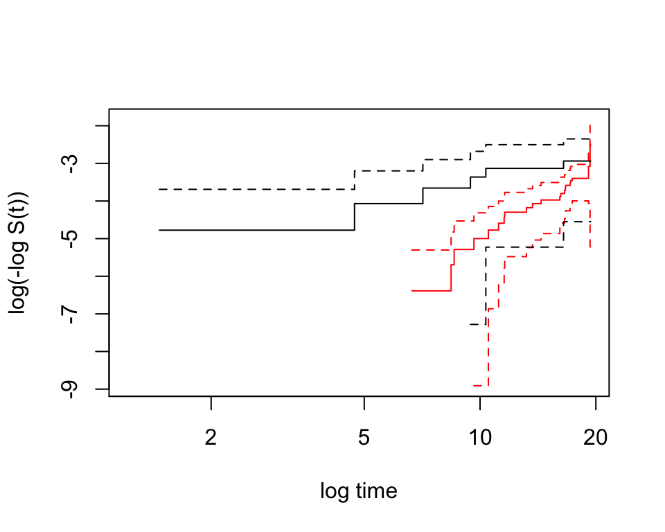
圖 87.5: Non-paramatric plot to investigate whether the Weibull model fit the data appropriate
用 Weibull 分布模型的結果,繪制兩個 job grade 在 5 個不同年齡層次的估計生存概率曲線:
whl.weibull <- survreg(Surv(time, chd) ~ as.factor(grade) + as.factor(agecat), dist = "weibull", data = whitehall)
plot(predict(whl.weibull, newdata = list(grade = 1, agecat = 1),  type = "quantile", p = seq(0.01, 0.99, by = 0.01)), seq(0.99, 0.01, by = -0.01), type = "l", lwd = 2, col = "red",
     xlab = "Time", ylab = "Survivor function: S(t)", xlim = c(0,20), ylim = c(0.5, 1))
lines(predict(whl.weibull, newdata = list(grade = 2, agecat = 1),  type = "quantile", p = seq(0.01, 0.99, by = 0.01)), seq(0.99, 0.01, by = -0.01), type = "l", lwd = 2, lty = 2, col = "red")

lines(predict(whl.weibull, newdata = list(grade = 1, agecat = 2),  type = "quantile", p = seq(0.01, 0.99, by = 0.01)), seq(0.99, 0.01, by = -0.01), type = "l", lwd = 2, lty = 1, col = "green")
lines(predict(whl.weibull, newdata = list(grade = 2, agecat = 2),  type = "quantile", p = seq(0.01, 0.99, by = 0.01)), seq(0.99, 0.01, by = -0.01), type = "l", lwd = 2, lty = 2, col = "green")

lines(predict(whl.weibull, newdata = list(grade = 1, agecat = 3),  type = "quantile", p = seq(0.01, 0.99, by = 0.01)), seq(0.99, 0.01, by = -0.01), type = "l", lwd = 2, lty = 1, col = "black")
lines(predict(whl.weibull, newdata = list(grade = 2, agecat = 3),  type = "quantile", p = seq(0.01, 0.99, by = 0.01)), seq(0.99, 0.01, by = -0.01), type = "l", lwd = 2, lty = 2, col = "black")

lines(predict(whl.weibull, newdata = list(grade = 1, agecat = 4),  type = "quantile", p = seq(0.01, 0.99, by = 0.01)), seq(0.99, 0.01, by = -0.01), type = "l", lwd = 2, lty = 1, col = "orange")
lines(predict(whl.weibull, newdata = list(grade = 2, agecat = 4),  type = "quantile", p = seq(0.01, 0.99, by = 0.01)), seq(0.99, 0.01, by = -0.01), type = "l", lwd = 2, lty = 2, col = "orange")

lines(predict(whl.weibull, newdata = list(grade = 1, agecat = 5),  type = "quantile", p = seq(0.01, 0.99, by = 0.01)), seq(0.99, 0.01, by = -0.01), type = "l", lwd = 2, lty = 1, col = "blue")
lines(predict(whl.weibull, newdata = list(grade = 2, agecat = 5),  type = "quantile", p = seq(0.01, 0.99, by = 0.01)), seq(0.99, 0.01, by = -0.01), type = "l", lwd = 2, lty = 2, col = "blue")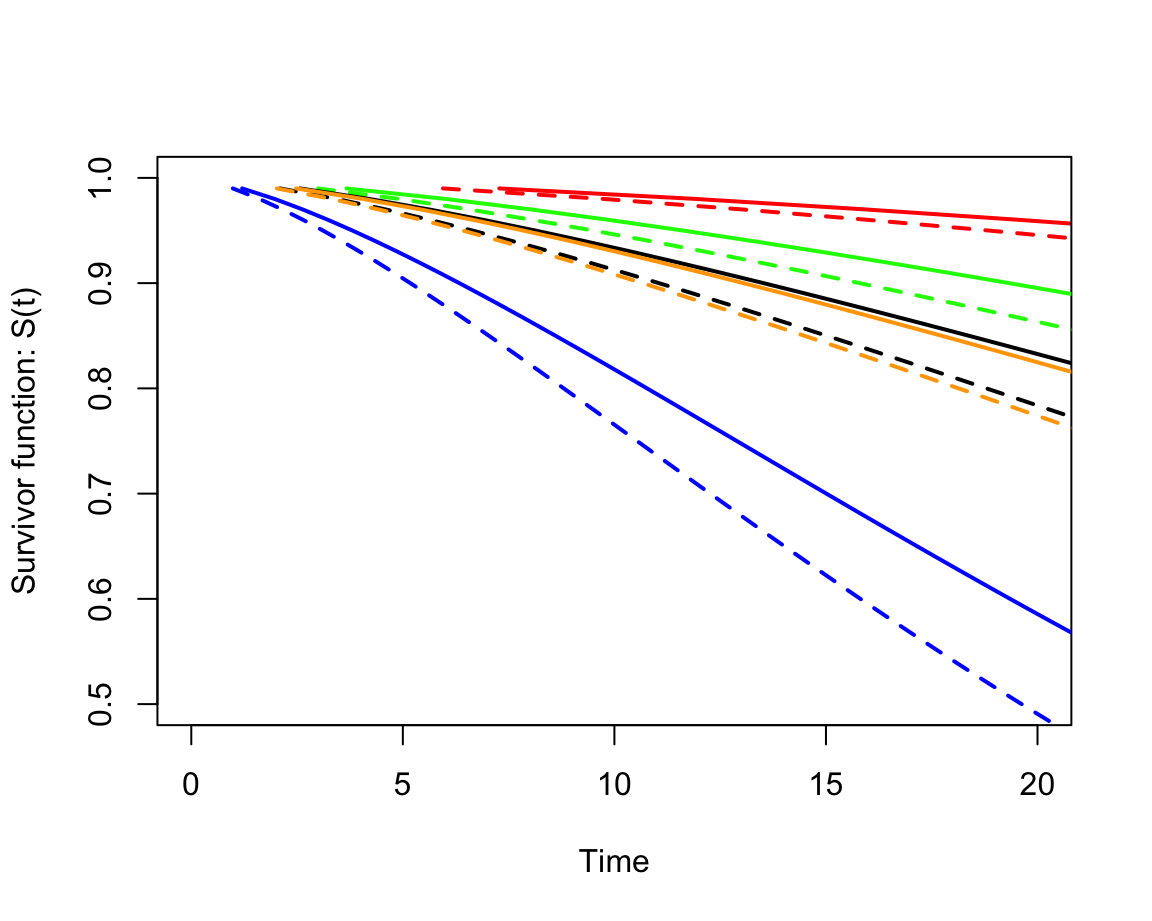
圖 87.6: The estimated survivor curves from the Weibull model in each job and age-at-entry category
下面把隨訪時間按照 5 到 20 年每間隔五年的方法把所有患者的追蹤時間截斷成4個部分。然後用指數分布回歸模型擬合數據,這也是一種放鬆恆定事件發生率這一前提條件的方法:
whl.split <- survSplit(Surv(time, chd) ~ ., whitehall, cut = c(0, 5, 10, 15, 20), start = "time0", episode = "fuband")

with(whitehall, whitehall[id == 5038,])
## # A tibble: 1 × 16
## id all chd sbp chol grade4 smok agein grade cholgrp sbpgrp timein timeout timebth time
## <dbl> <dbl> <dbl> <dbl> <dbl> <dbl> <dbl> <dbl> <dbl> <dbl> <dbl> <dbl> <dbl> <dbl> <dbl>
## 1 5038 0 0 147 295 2 3 51.4 1 4 3 -840. 6239. -19630. 19.4
## # … with 1 more variable: agecat <int>## id all sbp chol grade4 smok agein grade cholgrp sbpgrp timein timeout timebth
## 9 5038 0 147 295 2 3 51.444218 1 4 3 -840.01318 6238.9795 -19630.013
## 10 5038 0 147 295 2 3 51.444218 1 4 3 -840.01318 6238.9795 -19630.013
## 11 5038 0 147 295 2 3 51.444218 1 4 3 -840.01318 6238.9795 -19630.013
## 12 5038 0 147 295 2 3 51.444218 1 4 3 -840.01318 6238.9795 -19630.013
## agecat time0 time chd fuband
## 9 2 0 5.000000 0 2
## 10 2 5 10.000000 0 3
## 11 2 10 15.000000 0 4
## 12 2 15 19.381226 0 5whl.split.exp <- flexsurvreg(Surv(time0, time, chd) ~ as.factor(grade) + as.factor(agecat) +
as.factor(fuband), dist = "exponential", data = whl.split)
whl.split.exp## Call:
## flexsurvreg(formula = Surv(time0, time, chd) ~ as.factor(grade) +
## as.factor(agecat) + as.factor(fuband), data = whl.split,
## dist = "exponential")
##
## Estimates:
## data mean est L95% U95% se exp(est) L95%
## rate NA 0.001059 0.000627 0.001788 0.000283 NA NA
## as.factor(grade)2 0.266742 0.286099 -0.057633 0.629832 0.175377 1.331225 0.943996
## as.factor(agecat)2 0.218258 0.970919 0.464910 1.476929 0.258173 2.640371 1.591871
## as.factor(agecat)3 0.194422 1.477681 1.003971 1.951391 0.241693 4.382770 2.729098
## as.factor(agecat)4 0.114967 1.529719 0.998873 2.060564 0.270845 4.616879 2.715221
## as.factor(agecat)5 0.016053 2.562203 1.824200 3.300206 0.376539 12.964346 6.197837
## as.factor(fuband)3 0.261716 0.628789 0.153466 1.104112 0.242516 1.875338 1.165868
## as.factor(fuband)4 0.242744 0.783803 0.307212 1.260394 0.243163 2.189785 1.359630
## as.factor(fuband)5 0.223610 1.074270 0.569018 1.579521 0.257786 2.927854 1.766532
## U95%
## rate NA
## as.factor(grade)2 1.877295
## as.factor(agecat)2 4.379475
## as.factor(agecat)3 7.038471
## as.factor(agecat)4 7.850399
## as.factor(agecat)5 27.118213
## as.factor(fuband)3 3.016545
## as.factor(fuband)4 3.526812
## as.factor(fuband)5 4.852629
##
## N = 6167, Events: 154, Censored: 6013
## Total time at risk: 27605.371
## Log-likelihood = -904.07753, df = 9
## AIC = 1826.1551我們用指數分布回歸擬合的生存時間模型,其實還可以用泊鬆回歸模型來做,結果也是一樣的:
whl.poi <- glm(chd ~ as.factor(grade), family = poisson(link = log), offset = log(time), data = whitehall)
summary(whl.poi)
##
## Call:
## glm(formula = chd ~ as.factor(grade), family = poisson(link = log),
## data = whitehall, offset = log(time))
##
## Deviance Residuals:
## Min 1Q Median 3Q Max
## -0.58433 -0.41268 -0.40212 -0.39440 3.55361
##
## Coefficients:
## Estimate Std. Error z value Pr(>|z|)
## (Intercept) -5.42052 0.10541 -51.4238 < 2.2e-16 ***
## as.factor(grade)2 0.68850 0.16351 4.2108 0.00002545 ***
## ---
## Signif. codes: 0 '***' 0.001 '**' 0.01 '*' 0.05 '.' 0.1 ' ' 1
##
## (Dispersion parameter for poisson family taken to be 1)
##
## Null deviance: 947.906 on 1676 degrees of freedom
## Residual deviance: 931.144 on 1675 degrees of freedom
## AIC: 1243.14
##
## Number of Fisher Scoring iterations: 6你可以回頭去和指數分布回歸的模型結果做個比較,他們的回歸系數估計和標準誤完全是一樣的。