第 74 章 隨機截距模型中加入共變量 random intercept model with covariates
這一章我們來把隨機截距模型加以擴展,在固定效應部分增加想要調整的共變量。
74.1 多元線性回歸模型的延伸
如果有一個含有兩個預測變量的多元線性回歸模型:
\[ \begin{equation} Y_{ij} = \beta_0 + \beta_1 X_{1ij} + \beta_2 X_{2ij} + \epsilon_{ij} \end{equation} \tag{74.1} \]
如果觀測數據內部具有嵌套式結構,也就是有些對象之間有相關性,有些對象之間沒有,那麼上面這個多元線性回歸模型的誤差項 \(\epsilon_{ij}\) 其實是不能被認爲相互獨立的,因爲數據中處以同一層的個體之間互相有關聯性 (屬於同一所學校的學生之間,同一所醫院的病人之間)。但是於此同時,我們不妨把最後的誤差項分成兩個部分
\[ \epsilon_{ij} = u_j + e_{ij} \]
其中,
- \(u_j\),是在隨機截距模型中用到的隨機截距部分,\(u_j \sim N(0, \sigma_u^2)\),它允許不同層的數據有自己的截距;
- \(e_{ij}\),是剝離掉層內相關 (等同於層間相異,intra-class correlation = between-class heterogeneity) 之後,剩餘的隨機殘差;
之後把式子 (74.1) 重新整理,就遇到了我們似曾相識的隨機截距模型:
\[ \begin{equation} Y_{ij} = (\beta_0 + u_j) + \beta_1 X_{1ij} + \beta_2 X_{2ij} + e_{ij} \end{equation} \tag{74.2} \]
這就是一個混合效應線性回歸模型 (linear mixed model)。其中,
- 固定效應部分的參數有 fixed effect parameters: \(\beta_0, \beta_1, \beta_2\);
- 隨機效應部分的參數有 random effect parameters: \(u_j, e_{ij}\)。
但是和之前的隨機截距模型不同的是,這裏我們在固定效應部分增加了兩個共變量 \(X_1, X_2\),所以從該模型作出的所有統計推斷,都是建立在以這兩個共變量爲條件的基礎之上的 (conditionally on \(\mathbf{X} = \{ X_1, X_2\}\))。所以對於 \(u_j, e_{ij}\),他們的前提條件就變成了:
- \(\text{E}(u_j|\mathbf{X} = \{ X_1, X_2\}) = 0\);
- \(\text{E}(e_{ij}|\mathbf{X} = \{ X_1, X_2, u_j\}) = 0\)。
根據這兩個條件,我們可以繼續得到:
- \(\text{E}(e_{ij} | \mathbf{X} = \{ X_1, X_2\}) = 0\);
- \(\text{E}(Y_{ij} | \mathbf{X} = \{ X_1, X_2\}) = \beta_0 + \beta_1X_{1ij} + \beta_2X_{2ij}\)
也就是說,這個包含了 \(u_j, e_{ij}\) 的多元線性回歸模型,其邊際模型 (marginal regression over \(u_j, e_{ij}\)) 還是一個線性回歸。
注意
- 模型的固定效應部分加入了多個共變量 \(\mathbf{X} = \{ X_1, X_2\}\) 之後,模型所估計的層內相關系數 (intra-class correlation, \(\lambda\)) 也成了以這些共變量爲條件的層內相關系數。
- \(u_j\) 這個層別隨機截距 (cluster-specific random intercept) 此時會囊括已知/未知的層水平的特徵 (class-level characteristics, i.e. unmeasured heterogeneity between clusters)。它會隨着你在模型中加入層水平的解釋變量而逐漸變小 (Its size will decrease as more explanatory variables for the cluster difference are included in the model)。
74.2 siblings 數據中新生兒體重的實例
在數據 silblings 中,研究者收集了來自 3978 名母親,8604 名新生兒出生體重 (g) 的數據。此外,該數據中還收集了這些新生兒的胎齡 (week),新生兒的性別,母親孕期的吸煙狀況,以及懷孕時母親的年齡。在這個數據裏,每個母親是該數據的第二階層 (level 2),每個母親的相關信息,就是屬於第二階層的層水平數據。每個新生兒的體重和相關數據,就是第一階層 (level 1) 數據,一個母親可能生 1-3 個嬰兒,這些來自同一個母親的新生兒之間很顯然不能視之爲相互獨立。研究者關心一個固定效應部分不包含其他共變量的隨機截距模型 (the Null Model),和固定效應部分增加了其他共變量的隨機截距模型 (the Full Model) 哪個更能解釋這個數據或者更好的擬合這個數據 (better fitting the data)。
下面就先把數據讀入 R,然後建立一個零模型 (the Null Model):
siblings <- read_dta("../backupfiles/siblings.dta")
M0 <- lme(fixed = birwt ~ 1, random  = ~ 1 | momid, data = siblings, method = "REML")
summary(M0)
## Linear mixed-effects model fit by REML
## Data: siblings
## AIC BIC logLik
## 130951.2 130972.38 -65472.601
##
## Random effects:
## Formula: ~1 | momid
## (Intercept) Residual
## StdDev: 368.35597 377.65768
##
## Fixed effects: birwt ~ 1
## Value Std.Error DF t-value p-value
## (Intercept) 3467.9688 7.1385551 4626 485.80822 0
##
## Standardized Within-Group Residuals:
## Min Q1 Med Q3 Max
## -6.2743063896 -0.4860193974 0.0035299789 0.5053550371 4.0503923656
##
## Number of Observations: 8604
## Number of Groups: 3978## Model df AIC BIC logLik Test L.Ratio p-value
## M0 1 3 130951.20 130972.38 -65472.601
## M0_fixed 2 2 132265.32 132279.44 -66130.660 1 vs 2 1316.1174 <.0001下一步,我們來對該數據擬合一個全模型 (the Full Model),我們可以先對兩個連續型變量 (胎齡,gestational age 和母親懷孕時年齡,maternal age) 進行適當的轉換,比方說把胎齡標準化成 38 周,懷孕時年齡標準化成 30 歲:
siblings <- siblings %>%
  mutate(c_gestat = gestat - 38, # centering gestational age to 38 weeks
         c_mage = mage - 30,  # centering maternal age to 30 years old
         male = factor(male, labels = c("female", "male")),
         smoke = factor(smoke, labels = c("Nonsmoker", "Smoker")))
#M_full <- lme(fixed = birwt ~ c_gestat + male + smoke + c_mage, random  = ~ 1 | momid, data = siblings, method = "REML")
M_full <- lmer(birwt ~ c_gestat + male + smoke + c_mage + (1 | momid), data = siblings, REML = TRUE)
library(lmerTest)
summary(M_full)
## Linear mixed model fit by REML. t-tests use Satterthwaite's method ['lmerModLmerTest']
## Formula: birwt ~ c_gestat + male + smoke + c_mage + (1 | momid)
## Data: siblings
##
## REML criterion at convergence: 128984.9
##
## Scaled residuals:
## Min 1Q Median 3Q Max
## -4.14590 -0.52884 -0.00868 0.53594 3.63288
##
## Random effects:
## Groups Name Variance Std.Dev.
## momid (Intercept) 99784 315.89
## Residual 118012 343.53
## Number of obs: 8604, groups: momid, 3978
##
## Fixed effects:
## Estimate Std. Error df t value Pr(>|t|)
## (Intercept) 3341.0957 8.6642 7084.5208 385.620 < 2.2e-16 ***
## c_gestat 85.4241 2.1607 7868.3663 39.535 < 2.2e-16 ***
## malemale 133.9476 8.8694 7121.4202 15.102 < 2.2e-16 ***
## smokeSmoker -239.9993 15.9794 7543.5486 -15.019 < 2.2e-16 ***
## c_mage 13.1579 1.0903 5400.3042 12.068 < 2.2e-16 ***
## ---
## Signif. codes: 0 '***' 0.001 '**' 0.01 '*' 0.05 '.' 0.1 ' ' 1
##
## Correlation of Fixed Effects:
## (Intr) c_gstt maleml smkSmk
## c_gestat -0.347
## malemale -0.535 0.038
## smokeSmoker -0.244 0.017 0.006
## c_mage 0.137 0.020 -0.001 0.145從全模型的結果報告中可以看出,固定效應部分加入的所有解釋變量都是有意義的。他們的含義如下:
c_gestat 85.42: 當模型中的其他變量保持不變時 (當模型中其他的變量被調整時),胎齡每增加一周,無論是同一個媽媽還是不同媽媽 (either from the same or another mother, i.e. in any cluster) 生下的新生兒的出生體重增加的期待值是 85.42 g。male 133.95: 新生兒的性別如果是男孩,無論是同一個媽媽還是不同媽媽生下的新生兒,他的出生體重會比女孩增加 133.95 g。
再看這兩個模型的隨機效應部分,無論是第二層級水平的層標準差 (cluster-level) 還是第一層級 (elementary-level) 的標準差都隨着固定效應部分加入新的解釋變量而變小。我們同樣可以用極大似然法 (ML) 擬合這兩個模型,其方差大小總結成下面的表格:
| Random Effect | Null Model | Full Model | Null Model | Full Model |
|---|---|---|---|---|
| \(\hat\sigma_u\) | 368.3558 | 315.8853 | 368.2864 | 315.7320 |
| \(\hat\sigma_e\) | 377.6577 | 343.5296 | 377.6579 | 343.4581 |
表格的右半部分總結的是使用極大似然法 (會偏小估計隨機效應方差),其實它們和 REML 法估計的結果相差不大。值得強調的是,由於 REML 法每次估計的數據是去除掉固定效應部分以後的隨機誤差部分的數據,所以當兩個用 REML 法估計的混合效應模型其固定效應部分不一致的時候,這兩個模型實際擬合了不同的數據,是不能使用 LRT 來比較兩個模型哪個更好的。
74.3 賦值予隨機效應成分
值得建議地,擬合了任何一個混合效應模型以後,需要盡量避免直接跳入結論陳述階段,而應當先對模型是否符合其假定的前提條件進行模型診斷。而且,對模型的擬合後截距及其層級隨機效應 (cluster random effect) 進行視覺化展現變得十分有用。
總體來說,有兩種方法可以用於估計並提取這些擬合值 – ML 和 Empirical Bayes (EB)。
74.3.1 簡單預測 simple prediction
和簡單線性回歸模型一樣,我們可以計_算模型的預測值和觀測值之間的差,獲得一個包含了兩個隨機效應成分的量:
\[ \begin{aligned} Y_{ij} & = \beta_0 + \beta_1X_{1ij} + u_j + e_{ij} \\ \Rightarrow Y_{ij} & = \beta_0 + \beta_1X_{1ij} + \epsilon_{ij} \\ \Rightarrow \hat\epsilon_{ij} & = Y_{ij} - (\hat\beta_0 + \beta_1X_{1ij}) \end{aligned} \]
那麼最簡單的方法就是計算了這個隨機效應成分的混合體之後,對其取平均值,作爲 \(u_j\) 的簡單估計:
M_full <- lme(fixed = birwt ~ c_gestat + male + smoke + c_mage, random  = ~ 1 | momid,
              data = siblings, method = "REML")

siblings$yhat <- M_full$fitted[,1]
siblings <- siblings %>%
  mutate(res = birwt- yhat)
Mean_siblings <- ddply(siblings, ~momid, summarise, uhat = mean(res))
Mean_siblings[Mean_siblings$momid == 14,]
## momid uhat
## 1 14 105.124## # A tibble: 3 × 5
## momid gestat birwt yhat res
## <dbl> <dbl> <dbl> <dbl> <dbl>
## 1 14 24 2790 1961. 829.
## 2 14 42 2693 3512. -819.
## 3 14 39 3600 3295. 305.找到編號 14 號的母親,她有三個孩子被研究者記錄到,他們中有的孩子使用該模型計算的擬合值 (fitted value = yhat) 並不準確。在調整了胎齡,嬰兒性別,母親的吸煙狀況,和母親懷孕時年齡後,該母親生的孩子,和該隊列的總體平均值 (overall mean) 相比較,其偏差達到了 105.12 g。
我們可以對每個母親的擬合偏差做總結歸納:
Mean_siblings %>%
  summarise(Mean_uhat = mean(uhat),
            sd_uhat = sd(uhat),
            min_uhat = min(uhat),
            max_uhat = max(uhat))
## Mean_uhat sd_uhat min_uhat max_uhat
## 1 -0.5115952 395.0677 -1386.9365 1772.7215可見這 3978 名母親總體的擬合偏差的均值爲 -0.511,接近零。且它的標準差接近 400。這樣一種直接利用觀測值和擬合值之差做曾內平均的方法被叫做極大似然法 ML,這樣計算獲得的平均偏差被標記爲 \(\hat u_j^{\text{ML}}\)
74.3.2 EB 預測值
EB 法 (經驗貝葉斯法) 也一樣要利用擬合模型後的 \(\beta\) 來計算獲得層殘差 (cluster level residuals)。但是用 EB 法時我們還再使用層殘差的一個前提條件: \(u_j \sim N(0, \sigma_u^2)\)。在線性隨機截距模型中,EB 法計算的層級殘差和簡單法計算的層殘差之間有如下的簡單轉換關系:
\[ \hat u_j^{\text{EB}} = \hat R_j\hat u_j^{\text{ML}} \]
其中 \(\hat R_j\) 被定義爲 ML 法計算層級殘差的可靠性 (reliability of \(\hat u_j^{\text{ML}}\)),它是一個包含了層級方差和個人水平方差的方程:
\[ \hat R_j = \frac{\hat\sigma_u^2}{\hat\sigma_u^2 + \sigma_e^2/n_j} = \hat w_j \hat \sigma_u^2 \]
其中 \(\hat w_j\) 是之前在章節 73.4.1 定義的權重。這個 \(\hat R_j\) 又被叫做是收縮因子 (shrinkage factor),因爲它取值是在 0 到 1 之間,所以它會把 ML 法計算獲得的層級誤差按照收縮銀子比例收縮變小。當 \(\sigma_u\) 本身比較小,或者個體的隨機誤差大 \(\sigma_e\),或者層內樣本量小 \(n_j\) 時收縮因子的作用更大。
此時,預測誤差 \((\hat u_j^{\text{EB}} - u_j)\) 才是我們能夠從觀測數據以及模型中獲得的均值爲零方差又最小的殘差。所以 \(\hat u_j^{\text{EB}}\) 又被稱爲 \(\text{Best linear unbiased predictors, BLUP}\)。
第二層級殘差的方差是:
\[ R_j\hat \sigma_u^2 \]
74.4 混合效應模型的診斷
辛苦計算了 BLUP 之後,就可以拿它,和模型的標準化殘差來對模型作出一定的診斷。由於計算獲得的 BLUP 方差不齊,要先對其標準化之後再作正態圖:
# the standardized

n_child <- siblings %>% count(momid, sort = TRUE)
Mean_siblings <- merge(Mean_siblings, n_child, by = "momid")

Mean_siblings <- Mean_siblings %>%
  mutate(# extract the random effect (EB) residuals at level 2
         uhat_eb = ranef(M_full)$`(Intercept)`,
         # shrinkage factor
         R = 315.7338^2/(315.7338^2 + (343.4572^2)/n),
         # Empirical Bayes prediction of variance of uhat
         var_eb = R*(315.7338^2),
         # standardize the EB uhat
         uhat_st = uhat_eb/sqrt(var_eb)
  )

# 計算每個個體的標準化殘差

siblings$ehat <- residuals(M_full, level = 1, type = "normalized")
圖 74.1: Histogram and Q-Q plot of cluster (mother) level unstandardized residuals for the intercept
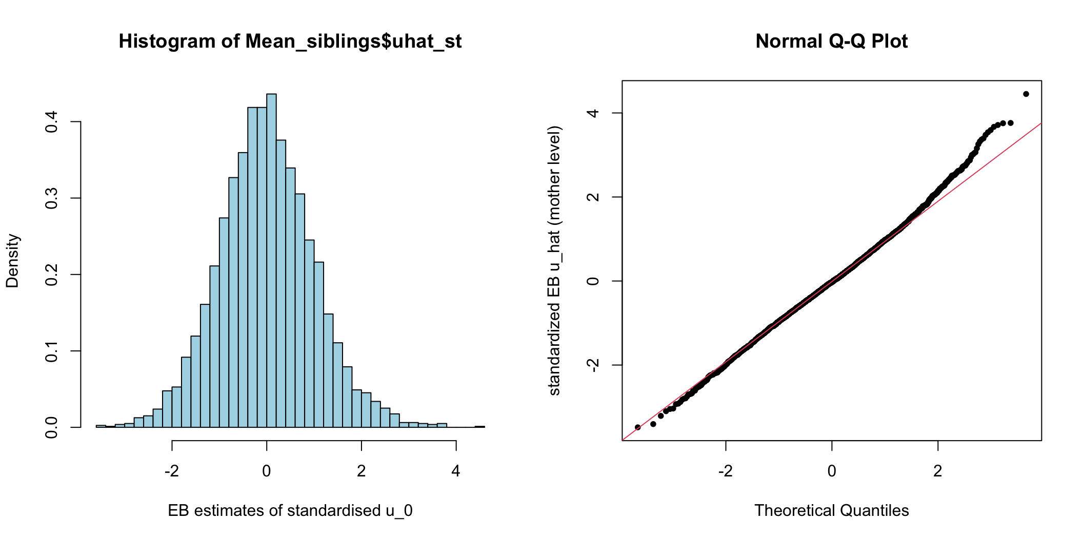
圖 74.2: Histogram and Q-Q plot of cluster (mother) level standardized residuals for the intercept
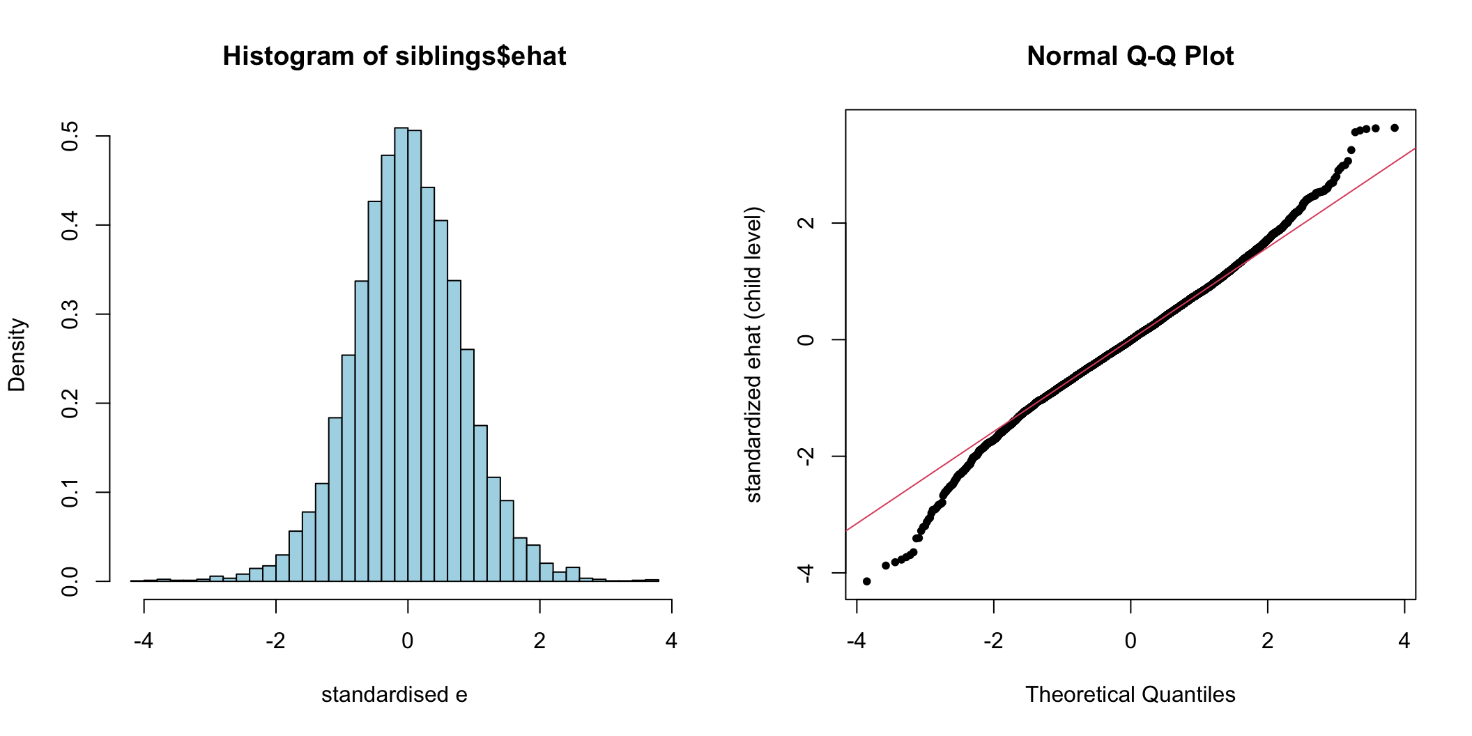
圖 74.3: Histogram and Q-Q plot of individual (pupil) level standardized residuals for the intercept
這些正態圖,主要用於輔助尋找看哪裏有異常值 (outliers)。
74.5 第二層級 (cluster level/level 2) 的協方差
還是這個 siblings 數據中,關於母親的數據在該母親生的孩子中是保持不變的,比如有人種 (black),母親受教育情況 (hsgrad),和母親的婚姻狀況 (married)。因爲這些變量屬於解釋第二層級 (level 2) 的變量,加入這些變量在固定效應部分只能解釋層間的方差 (between clusters variance):
siblings <- siblings %>%
  mutate(black = factor(black, labels = c("No", "Yes")),
         hsgrad = factor(hsgrad, labels = c("No", "Yes")),
         married = factor(married, labels = c("No", "yes")))

M_full1 <- lmer(birwt ~ c_gestat + male + smoke + c_mage + black + married + hsgrad + (1 | momid),
                data = siblings, REML = TRUE)
summary(M_full1)
## Linear mixed model fit by REML. t-tests use Satterthwaite's method ['lmerModLmerTest']
## Formula: birwt ~ c_gestat + male + smoke + c_mage + black + married + hsgrad + (1 | momid)
## Data: siblings
##
## REML criterion at convergence: 128884.7
##
## Scaled residuals:
## Min 1Q Median 3Q Max
## -4.19306 -0.53217 -0.01244 0.54116 3.65296
##
## Random effects:
## Groups Name Variance Std.Dev.
## momid (Intercept) 96846 311.20
## Residual 118053 343.59
## Number of obs: 8604, groups: momid, 3978
##
## Fixed effects:
## Estimate Std. Error df t value Pr(>|t|)
## (Intercept) 3297.4611 23.3036 4601.1760 141.4998 < 2.2e-16 ***
## c_gestat 84.4555 2.1584 7887.4033 39.1281 < 2.2e-16 ***
## malemale 133.7891 8.8514 7160.4073 15.1150 < 2.2e-16 ***
## smokeSmoker -227.9418 16.3323 7674.0013 -13.9565 < 2.2e-16 ***
## c_mage 11.0375 1.1412 5488.4090 9.6716 < 2.2e-16 ***
## blackYes -177.8954 25.9709 3912.4116 -6.8498 8.554e-12 ***
## marriedyes 61.1716 22.2791 4164.2316 2.7457 0.006064 **
## hsgradYes -4.2118 13.9792 3949.6037 -0.3013 0.763211
## ---
## Signif. codes: 0 '***' 0.001 '**' 0.01 '*' 0.05 '.' 0.1 ' ' 1
##
## Correlation of Fixed Effects:
## (Intr) c_gstt maleml smkSmk c_mage blckYs mrrdys
## c_gestat -0.111
## malemale -0.204 0.038
## smokeSmoker -0.287 0.009 0.008
## c_mage 0.222 0.034 -0.004 0.071
## blackYes -0.377 0.041 0.007 0.064 0.036
## marriedyes -0.914 -0.025 0.007 0.227 -0.230 0.348
## hsgradYes -0.165 0.011 -0.012 -0.044 0.172 -0.046 0.016加入了第二層級協變量之後, \(\sigma^2_u = 96845.79\),相比沒加之前的小了一些 \((\sigma^2_{u} = 99784)\)。但是 \(\sigma^2_e\) 幾乎保持不變。
74.6 層內層間效應估計
如有某個想加入模型的變量是屬於第一層級的,例如 siblings 數據中的胎齡,即使是同一個媽媽生的嬰兒,其出生時的胎齡也是各不相同。但是這樣在模型輸出的報告中,胎齡這一變量的估計量其實是其他變量保持不變時,每增加一周胎兒對不論是同一個母親還是不同母親生的嬰兒的出生體重的影響,怎樣才能把同一母親不同胎齡的影響 (within effect) 和不同母親不同胎齡的影響 (between effect) 給區分出來呢?
其實很簡單,我們來把胎齡這個變量做個分解:
\[ Y_{ij} = \beta_0 + \beta_{1B} \bar{X}_{\cdot j} + \beta_{1W} (X_{ij} - \bar{X}_{\cdot j}) + u_j + e_{ij} \]
把胎齡這個變量分解成 \(\bar{X}_{\cdot j}\) (每個母親生的嬰兒的平均胎齡),和 \(X_{ij} - \bar{X}_{\cdot j}\) (每個母親內,每個胎兒的胎齡和平均胎齡之差) 兩個部分,就解決了區分層間效應 \((\beta_{1B})\) 和層內效應 \((\beta_{1W})\)。 的方法。下面的模型在固定效應部分只使用了胎齡一個變量 (爲了這裏輸出報告簡潔明了):
## Linear mixed model fit by REML. t-tests use Satterthwaite's method ['lmerModLmerTest']
## Formula: birwt ~ c_gestat + (1 | momid)
##    Data: siblings
##
## REML criterion at convergence: 129638.4
##
## Scaled residuals:
##      Min       1Q   Median       3Q      Max
## -3.95662 -0.52950  0.00662  0.52638  3.98718
##
## Random effects:
##  Groups   Name        Variance Std.Dev.
##  momid    (Intercept) 113073   336.26
##  Residual             124282   352.54
## Number of obs: 8604, groups:  momid, 3978
##
## Fixed effects:
##              Estimate Std. Error        df t value  Pr(>|t|)
## (Intercept) 3358.5435     7.1841 4956.3637 467.497 < 2.2e-16 ***
## c_gestat      83.7325     2.2314 7785.2519  37.525 < 2.2e-16 ***
## ---
## Signif. codes:  0 '***' 0.001 '**' 0.01 '*' 0.05 '.' 0.1 ' ' 1
##
## Correlation of Fixed Effects:
##          (Intr)
## c_gestat -0.406
當把胎齡作爲一個變量放進模型的固定效應部分時,不論是不是同一個母親生下的胎兒,只要胎齡每增加一周,出生體重就增加 83.7 g。下一個模型中,我們來把胎齡這個變量分解成層間變量和層內變量:
Mean_gestat <- ddply(siblings, ~ momid, summarise, mean_gestat = mean(gestat))
# 把每個母親的胎兒胎齡均值 (level 2 mean) 賦予原有的數據中
avegest <- NULL
for (i in 1:3978){
  avegest <- c(avegest, rep(Mean_gestat$mean_gestat[i], with(siblings, table(momid))[i]))
}
siblings$avegest <- avegest
rm(avegest)
# 計算層內胎兒胎齡與其層均值的差異
siblings <- siblings %>%
  mutate(c_avegest = avegest - 38,
         difgest = gestat - avegest)

siblings[siblings$momid == 14,c(1,2,5,6,18:20)]
## # A tibble: 3 × 7
## momid idx gestat birwt avegest c_avegest difgest
## <dbl> <dbl> <dbl> <dbl> <dbl> <dbl> <dbl>
## 1 14 1 24 2790 35 -3 -11
## 2 14 2 42 2693 35 -3 7
## 3 14 3 39 3600 35 -3 4# 下面用 c_avegest 和 difgest 代替 gestat 放入同樣模型的固定效應部分
M_gestat_sep <- lmer(birwt ~ c_avegest + difgest + (1 | momid), data = siblings, REML = TRUE)
summary(M_gestat_sep)## Linear mixed model fit by REML. t-tests use Satterthwaite's method ['lmerModLmerTest']
## Formula: birwt ~ c_avegest + difgest + (1 | momid)
## Data: siblings
##
## REML criterion at convergence: 129557.3
##
## Scaled residuals:
## Min 1Q Median 3Q Max
## -4.02183 -0.52451 0.00937 0.52315 3.98953
##
## Random effects:
## Groups Name Variance Std.Dev.
## momid (Intercept) 111117 333.34
## Residual 123670 351.67
## Number of obs: 8604, groups: momid, 3978
##
## Fixed effects:
## Estimate Std. Error df t value Pr(>|t|)
## (Intercept) 3320.0084 8.3833 3974.3076 396.026 < 2.2e-16 ***
## c_avegest 113.2183 4.0294 3996.5078 28.098 < 2.2e-16 ***
## difgest 70.9350 2.6655 4626.8919 26.613 < 2.2e-16 ***
## ---
## Signif. codes: 0 '***' 0.001 '**' 0.01 '*' 0.05 '.' 0.1 ' ' 1
##
## Correlation of Fixed Effects:
## (Intr) c_vgst
## c_avegest -0.628
## difgest 0.000 0.000把胎齡分解了以後,從模型的輸出結果可以看出,層間效應 113 g (不同的母親),要大於層內效應 70.9 g (同一母親不同胎兒)。
比較分解胎齡以後的模型 M_gestat_sep 和把胎齡作爲一個變量的模型 M_gestat 哪個更優,可以有兩種檢驗法:
## Data: siblings
## Models:
## M_gestat: birwt ~ c_gestat + (1 | momid)
## M_gestat_sep: birwt ~ c_avegest + difgest + (1 | momid)
##              npar    AIC    BIC   logLik deviance  Chisq Df Pr(>Chisq)
## M_gestat        4 129656 129684 -64823.7   129648
## M_gestat_sep    5 129581 129617 -64785.6   129571 76.219  1 < 2.22e-16 ***
## ---
## Signif. codes: 0 '***' 0.001 '**' 0.01 '*' 0.05 '.' 0.1 ' ' 1## Linear hypothesis test
##
## Hypothesis:
## c_avegest - difgest = 0
##
## Model 1: restricted model
## Model 2: birwt ~ c_avegest + difgest + (1 | momid)
##
## Df Chisq Pr(>Chisq)
## 1
## 2 1 76.5998 < 2.22e-16 ***
## ---
## Signif. codes: 0 '***' 0.001 '**' 0.01 '*' 0.05 '.' 0.1 ' ' 1無論是哪種檢驗,都告訴我們把胎齡分解了的模型更好。了解更多層內層間回歸模型,參照 (Mann, De Stavola, and Leon 2004)。
74.7 到底選擇固定還是混合模型?
目前爲止我們討論了嵌套式數據可以使用固定效應模型分析,也可以使用混合效應模型來擬合,那麼到底你該選擇哪個來解釋你的數據呢? 選擇模型永遠是一個很難回答的問題。哪種模型更加恰當 (appropriate) 其實要取決於你的數據結構,分層的數據的話層的數量是不是足夠多?以及最重要的,你的**分析目的*。
- 如果模型中想分析的層/羣組,可以被視爲唯一的實體 (uniqe entity,例如不同的種族),而且我們希望從模型來獲得對不同種羣或者不同個體中每一個個體的估計,那麼固定效應模型是合適的。
- 如果層/羣組其實是人羣中的樣本 (samples from a real population,如例題中的母親層級,人羣衆可以有許許多多的母親),我們打算從這個模型的結果去推論整個人羣,那麼隨機效應模型才是最合適的。
- 如果說層級本身的樣本量 (n of clusters) 太小,那麼強行使用混合效應模型的話會導致隨機效應的估計結果十分地低效,甚至沒有意義; 當然如果你的混合效應模型關心的是固定效應部分,那麼增加一些層級隨機效應應該也能達到提升統計估計效率的目的。
- 如果我們關心的是層級協變量的效應,那麼隨機效應模型是唯一的選擇。
74.8 Practical Hierarchical 03
74.8.1 把 High-school-and-Beyond 數據讀入 R 中。
hsb_selected <- read_dta("../backupfiles/hsb_selected.dta")
length(unique(hsb_selected$schoolid)) ## number of school = 160
## [1] 160## create a subset data with only the first observation of each school
hsb <- hsb_selected[!duplicated(hsb_selected$schoolid), ]
## about 44 % of the schools are Catholic schools
with(hsb, tab1(sector, graph = FALSE, decimal = 2))## sector :
## Frequency Percent Cum. percent
## 0 90 56.25 56.25
## 1 70 43.75 100.00
## Total 160 100.00 100.00## among all the schools, average school size is 1098
hsb %>%
summarise(N = n(),
Mean = mean(size),
sd_size = sd(size),
min_size = min(size),
max_size = max(size))## # A tibble: 1 × 5
## N Mean sd_size min_size max_size
## <int> <dbl> <dbl> <dbl> <dbl>
## 1 160 1098. 630. 100 2713## among all the pupils, about 53% are females
with(hsb_selected, tab1(female, graph = FALSE, decimal = 2))## female :
## Frequency Percent Cum. percent
## 0 3390 47.18 47.18
## 1 3795 52.82 100.00
## Total 7185 100.00 100.00## among all the pupils, about 27.5% are from ethnic minorities
with(hsb_selected, tab1(minority, graph = FALSE, decimal = 2))## minority :
## Frequency Percent Cum. percent
## 0 5211 72.53 72.53
## 1 1974 27.47 100.00
## Total 7185 100.00 100.0074.8.2 擬合兩個隨機截距模型 (ML, REML),結果變量用 mathach,解釋變量用 ses。觀察結果是否不同。
Fixed_reml <- lmer(mathach ~ ses + (1 | schoolid), data = hsb_selected, REML = TRUE)
summary(Fixed_reml)
## Linear mixed model fit by REML. t-tests use Satterthwaite's method ['lmerModLmerTest']
## Formula: mathach ~ ses + (1 | schoolid)
## Data: hsb_selected
##
## REML criterion at convergence: 46645.2
##
## Scaled residuals:
## Min 1Q Median 3Q Max
## -3.126073 -0.727203 0.021883 0.757717 2.919116
##
## Random effects:
## Groups Name Variance Std.Dev.
## schoolid (Intercept) 4.7682 2.1836
## Residual 37.0344 6.0856
## Number of obs: 7185, groups: schoolid, 160
##
## Fixed effects:
## Estimate Std. Error df t value Pr(>|t|)
## (Intercept) 12.65748 0.18799 148.30225 67.332 < 2.2e-16 ***
## ses 2.39020 0.10572 6838.07757 22.609 < 2.2e-16 ***
## ---
## Signif. codes: 0 '***' 0.001 '**' 0.01 '*' 0.05 '.' 0.1 ' ' 1
##
## Correlation of Fixed Effects:
## (Intr)
## ses 0.003Fixed_ml <- lmer(mathach ~ ses + (1 | schoolid), data = hsb_selected, REML = FALSE)
summary(Fixed_ml)## Linear mixed model fit by maximum likelihood . t-tests use Satterthwaite's method [lmerModLmerTest]
## Formula: mathach ~ ses + (1 | schoolid)
## Data: hsb_selected
##
## AIC BIC logLik deviance df.resid
## 46649.0 46676.5 -23320.5 46641.0 7181
##
## Scaled residuals:
## Min 1Q Median 3Q Max
## -3.12631 -0.72766 0.02200 0.75781 2.91860
##
## Random effects:
## Groups Name Variance Std.Dev.
## schoolid (Intercept) 4.7285 2.1745
## Residual 37.0298 6.0852
## Number of obs: 7185, groups: schoolid, 160
##
## Fixed effects:
## Estimate Std. Error df t value Pr(>|t|)
## (Intercept) 12.65762 0.18732 149.17601 67.572 < 2.2e-16 ***
## ses 2.39150 0.10569 6837.30522 22.627 < 2.2e-16 ***
## ---
## Signif. codes: 0 '***' 0.001 '**' 0.01 '*' 0.05 '.' 0.1 ' ' 1
##
## Correlation of Fixed Effects:
## (Intr)
## ses 0.003其實由於樣本量 (層數) 足夠多,兩個隨機截距模型給出的參數估計十分接近。
74.8.3 觀察學校類型是否爲天主教學校 sector 的分佈,把它加入剛擬合的兩個隨機截距模型,它們估計的隨機效應標準差 \(\hat\sigma_u\),和隨機誤差標準差 \(\hat\sigma_e\),和之前有什麼不同? “ML,REML” 的選用對結果有影響嗎?
Fixed_reml <- lmer(mathach ~ ses + factor(sector) + (1 | schoolid), data = hsb_selected, REML = TRUE)
summary(Fixed_reml)
## Linear mixed model fit by REML. t-tests use Satterthwaite's method ['lmerModLmerTest']
## Formula: mathach ~ ses + factor(sector) + (1 | schoolid)
## Data: hsb_selected
##
## REML criterion at convergence: 46611.2
##
## Scaled residuals:
## Min 1Q Median 3Q Max
## -3.148567 -0.731004 0.019288 0.753657 2.926345
##
## Random effects:
## Groups Name Variance Std.Dev.
## schoolid (Intercept) 3.685 1.9196
## Residual 37.037 6.0858
## Number of obs: 7185, groups: schoolid, 160
##
## Fixed effects:
## Estimate Std. Error df t value Pr(>|t|)
## (Intercept) 11.71891 0.22806 153.58417 51.3855 < 2.2e-16 ***
## ses 2.37471 0.10549 6738.85825 22.5110 < 2.2e-16 ***
## factor(sector)1 2.10084 0.34112 147.35739 6.1586 6.638e-09 ***
## ---
## Signif. codes: 0 '***' 0.001 '**' 0.01 '*' 0.05 '.' 0.1 ' ' 1
##
## Correlation of Fixed Effects:
## (Intr) ses
## ses 0.063
## fctr(sctr)1 -0.672 -0.091Fixed_ml <- lmer(mathach ~ ses + factor(sector) + (1 | schoolid), data = hsb_selected, REML = FALSE)
summary(Fixed_ml)## Linear mixed model fit by maximum likelihood . t-tests use Satterthwaite's method [lmerModLmerTest]
## Formula: mathach ~ ses + factor(sector) + (1 | schoolid)
## Data: hsb_selected
##
## AIC BIC logLik deviance df.resid
## 46616.4 46650.8 -23303.2 46606.4 7180
##
## Scaled residuals:
## Min 1Q Median 3Q Max
## -3.149152 -0.730912 0.019585 0.754184 2.925231
##
## Random effects:
## Groups Name Variance Std.Dev.
## schoolid (Intercept) 3.6219 1.9031
## Residual 37.0328 6.0855
## Number of obs: 7185, groups: schoolid, 160
##
## Fixed effects:
## Estimate Std. Error df t value Pr(>|t|)
## (Intercept) 11.71927 0.22651 155.49785 51.7396 < 2.2e-16 ***
## ses 2.37710 0.10544 6735.02962 22.5440 < 2.2e-16 ***
## factor(sector)1 2.10005 0.33875 149.11328 6.1994 5.285e-09 ***
## ---
## Signif. codes: 0 '***' 0.001 '**' 0.01 '*' 0.05 '.' 0.1 ' ' 1
##
## Correlation of Fixed Effects:
## (Intr) ses
## ses 0.064
## fctr(sctr)1 -0.672 -0.092可以看出,sector 變量在學校層面上都是沒有變化的,所以加它進入混合效應的固定部分,只會對隨機效應標準差 (within level/cluster/group error) \(\hat\sigma_u\) 的估計造成影響,隨機誤差標準差 \(\hat\sigma_e\) 則幾乎不受影響。同樣的 “ML, REML” 兩種方法對結果的影響微乎其微。
74.8.4 現在把學校規模 size 這一變量加入混合效應模型的固定效應部分,記得先把該變量中心化,並除以 100,會有助於對結果的解釋 (比平均值每增加100名學生)。仔細觀察模型結果中隨機效應標準差和隨機誤差標準殘差的變化。
hsb_selected <- hsb_selected %>%
  mutate(c_size = (size - with(hsb, mean(size)))/100)

Fixed_reml <- lmer(mathach ~ ses + factor(sector) + c_size + (1 | schoolid), data = hsb_selected, REML = TRUE)
summary(Fixed_reml)
## Linear mixed model fit by REML. t-tests use Satterthwaite's method ['lmerModLmerTest']
## Formula: mathach ~ ses + factor(sector) + c_size + (1 | schoolid)
## Data: hsb_selected
##
## REML criterion at convergence: 46613.2
##
## Scaled residuals:
## Min 1Q Median 3Q Max
## -3.142084 -0.732778 0.018257 0.755374 2.922664
##
## Random effects:
## Groups Name Variance Std.Dev.
## schoolid (Intercept) 3.6367 1.9070
## Residual 37.0345 6.0856
## Number of obs: 7185, groups: schoolid, 160
##
## Fixed effects:
## Estimate Std. Error df t value Pr(>|t|)
## (Intercept) 11.588378 0.238560 151.299116 48.5764 < 2.2e-16 ***
## ses 2.374876 0.105459 6721.908754 22.5194 < 2.2e-16 ***
## factor(sector)1 2.401175 0.379378 145.265475 6.3292 2.885e-09 ***
## c_size 0.053553 0.030198 148.968765 1.7734 0.07821 .
## ---
## Signif. codes: 0 '***' 0.001 '**' 0.01 '*' 0.05 '.' 0.1 ' ' 1
##
## Correlation of Fixed Effects:
## (Intr) ses fct()1
## ses 0.063
## fctr(sctr)1 -0.710 -0.086
## c_size -0.309 -0.009 0.447Fixed_ml <- lmer(mathach ~ ses + factor(sector) + c_size + (1 | schoolid), data = hsb_selected, REML = FALSE)
summary(Fixed_ml)## Linear mixed model fit by maximum likelihood . t-tests use Satterthwaite's method [lmerModLmerTest]
## Formula: mathach ~ ses + factor(sector) + c_size + (1 | schoolid)
## Data: hsb_selected
##
## AIC BIC logLik deviance df.resid
## 46615.3 46656.5 -23301.6 46603.3 7179
##
## Scaled residuals:
## Min 1Q Median 3Q Max
## -3.142725 -0.733277 0.018426 0.756191 2.920849
##
## Random effects:
## Groups Name Variance Std.Dev.
## schoolid (Intercept) 3.5444 1.8827
## Residual 37.0307 6.0853
## Number of obs: 7185, groups: schoolid, 160
##
## Fixed effects:
## Estimate Std. Error df t value Pr(>|t|)
## (Intercept) 11.589234 0.236144 154.101375 49.0769 < 2.2e-16 ***
## ses 2.378431 0.105389 6715.629474 22.5680 < 2.2e-16 ***
## factor(sector)1 2.399344 0.375458 147.837153 6.3904 2.035e-09 ***
## c_size 0.053456 0.029890 151.673273 1.7884 0.0757 .
## ---
## Signif. codes: 0 '***' 0.001 '**' 0.01 '*' 0.05 '.' 0.1 ' ' 1
##
## Correlation of Fixed Effects:
## (Intr) ses fct()1
## ses 0.064
## fctr(sctr)1 -0.710 -0.087
## c_size -0.309 -0.009 0.447增加了 size 進入混合效應模型的固定效應部分,對兩種參數估計方法輸出的結果 \((\hat\sigma_u, \hat\sigma_e)\) 並沒有太大的影響。
74.8.5 在模型的固定效應部分增加 size*sector 的交互作用項。觀察輸出結果中該交互作用項是否有意義。用什麼檢驗方法判斷這個交互作用項能否幫助模型更加擬合數據?
Fixed_reml <- lmer(mathach ~ ses + factor(sector)*c_size + (1 | schoolid), data = hsb_selected, REML = TRUE)
summary(Fixed_reml)
## Linear mixed model fit by REML. t-tests use Satterthwaite's method ['lmerModLmerTest']
## Formula: mathach ~ ses + factor(sector) * c_size + (1 | schoolid)
## Data: hsb_selected
##
## REML criterion at convergence: 46613.5
##
## Scaled residuals:
## Min 1Q Median 3Q Max
## -3.130458 -0.730487 0.018183 0.753342 2.922402
##
## Random effects:
## Groups Name Variance Std.Dev.
## schoolid (Intercept) 3.5594 1.8866
## Residual 37.0370 6.0858
## Number of obs: 7185, groups: schoolid, 160
##
## Fixed effects:
## Estimate Std. Error df t value Pr(>|t|)
## (Intercept) 11.665327 0.240290 149.376494 48.5469 < 2.2e-16 ***
## ses 2.377719 0.105409 6689.156861 22.5572 < 2.2e-16 ***
## factor(sector)1 2.618912 0.395270 140.853919 6.6256 6.788e-10 ***
## c_size 0.022185 0.034603 151.266432 0.6411 0.52241
## factor(sector)1:c_size 0.124462 0.069016 139.397370 1.8034 0.07349 .
## ---
## Signif. codes: 0 '***' 0.001 '**' 0.01 '*' 0.05 '.' 0.1 ' ' 1
##
## Correlation of Fixed Effects:
## (Intr) ses fct()1 c_size
## ses 0.063
## fctr(sctr)1 -0.611 -0.083
## c_size -0.351 -0.007 0.214
## fctr(sc)1:_ 0.176 -0.001 0.308 -0.501Fixed_ml <- lmer(mathach ~ ses + factor(sector)*c_size + (1 | schoolid), data = hsb_selected, REML = FALSE)
summary(Fixed_ml)## Linear mixed model fit by maximum likelihood . t-tests use Satterthwaite's method [lmerModLmerTest]
## Formula: mathach ~ ses + factor(sector) * c_size + (1 | schoolid)
## Data: hsb_selected
##
## AIC BIC logLik deviance df.resid
## 46614.0 46662.1 -23300.0 46600.0 7178
##
## Scaled residuals:
## Min 1Q Median 3Q Max
## -3.130886 -0.730494 0.017706 0.753635 2.919879
##
## Random effects:
## Groups Name Variance Std.Dev.
## schoolid (Intercept) 3.4378 1.8541
## Residual 37.0338 6.0855
## Number of obs: 7185, groups: schoolid, 160
##
## Fixed effects:
## Estimate Std. Error df t value Pr(>|t|)
## (Intercept) 11.666606 0.237019 153.063389 49.2222 < 2.2e-16 ***
## ses 2.382601 0.105316 6679.214135 22.6234 < 2.2e-16 ***
## factor(sector)1 2.616394 0.389730 144.122856 6.7134 4.063e-10 ***
## c_size 0.021983 0.034135 155.039559 0.6440 0.52052
## factor(sector)1:c_size 0.124598 0.068044 142.600213 1.8311 0.06917 .
## ---
## Signif. codes: 0 '***' 0.001 '**' 0.01 '*' 0.05 '.' 0.1 ' ' 1
##
## Correlation of Fixed Effects:
## (Intr) ses fct()1 c_size
## ses 0.064
## fctr(sctr)1 -0.611 -0.084
## c_size -0.351 -0.007 0.214
## fctr(sc)1:_ 0.176 -0.001 0.307 -0.502在兩個估計方法的報告中,交互作用項均不具有統計學意義。
74.8.6 把上面八個模型估計的隨機效應標準差,和隨機誤差標準差總結成表格,它們之間有什麼規律嗎?
| Model with | \(\sigma_u\) | \(\sigma_e\) | \(\sigma_u\) | \(\sigma_e\) |
|---|---|---|---|---|
| ses | 2.184 | 6.085 | 2.175 | 6.085 |
| ses & sector | 1.920 | 6.086 | 1.903 | 6.086 |
| ses, size & sector | 1.907 | 6.086 | 1.883 | 6.085 |
|
ses, size & sector & size*sector |
1.887 | 6.086 | 1.854 | 6.086 |
\(\hat\sigma_e\) 幾乎在所有模型的估計中都保持不變。因爲我們在固定效應中增加的共變量在學校層面 (level 2) 都是一樣的。也就是說對於同一學校的學生,新增的共變量是一模一樣沒有變化的,所以在個人水平 (level 1) 的隨機效應幾乎不會發生變化。且注意到 “ML” 極大似然法估計的隨機效應標準差比 “REML” 限制性極大似然估計法給出的結果略小 1% 左右。
74.8.7 在混合效應模型的固定效應部分增加學生性別 female,和學生是否是少數族裔 minority 兩個變量。再觀察 \(\hat\sigma_u, \hat\sigma_e\) 是否發生變化?
Fixed_reml <- lmer(mathach ~ ses + factor(sector) + c_size + factor(female) + factor(minority) + (1 | schoolid), data = hsb_selected, REML = TRUE)
summary(Fixed_reml)
## Linear mixed model fit by REML. t-tests use Satterthwaite's method ['lmerModLmerTest']
## Formula: mathach ~ ses + factor(sector) + c_size + factor(female) + factor(minority) +
## (1 | schoolid)
## Data: hsb_selected
##
## REML criterion at convergence: 46336.4
##
## Scaled residuals:
## Min 1Q Median 3Q Max
## -3.28599 -0.71963 0.03760 0.75553 2.88323
##
## Random effects:
## Groups Name Variance Std.Dev.
## schoolid (Intercept) 2.1692 1.4728
## Residual 35.9184 5.9932
## Number of obs: 7185, groups: schoolid, 160
##
## Fixed effects:
## Estimate Std. Error df t value Pr(>|t|)
## (Intercept) 12.944772 0.217832 217.526187 59.4254 < 2.2e-16 ***
## ses 2.059675 0.105073 6543.507287 19.6024 < 2.2e-16 ***
## factor(sector)1 2.731292 0.310817 143.786918 8.7875 4.206e-15 ***
## c_size 0.076372 0.024802 148.489663 3.0793 0.002472 **
## factor(female)1 -1.252053 0.160241 5716.966427 -7.8135 6.572e-15 ***
## factor(minority)1 -3.098421 0.200627 3527.351887 -15.4437 < 2.2e-16 ***
## ---
## Signif. codes: 0 '***' 0.001 '**' 0.01 '*' 0.05 '.' 0.1 ' ' 1
##
## Correlation of Fixed Effects:
## (Intr) ses fctr(s)1 c_size fctr(f)1
## ses 0.000
## fctr(sctr)1 -0.624 -0.116
## c_size -0.265 -0.025 0.448
## factr(fml)1 -0.390 0.060 0.005 0.018
## fctr(mnrt)1 -0.206 0.212 -0.080 -0.074 0.011Fixed_ml <- lmer(mathach ~ ses + factor(sector) + c_size + factor(female) + factor(minority) + (1 | schoolid), data = hsb_selected, REML = FALSE)
summary(Fixed_ml)## Linear mixed model fit by maximum likelihood . t-tests use Satterthwaite's method [lmerModLmerTest]
## Formula: mathach ~ ses + factor(sector) + c_size + factor(female) + factor(minority) +
## (1 | schoolid)
## Data: hsb_selected
##
## AIC BIC logLik deviance df.resid
## 46338 46393 -23161 46322 7177
##
## Scaled residuals:
## Min 1Q Median 3Q Max
## -3.28718 -0.71993 0.03838 0.75632 2.88308
##
## Random effects:
## Groups Name Variance Std.Dev.
## schoolid (Intercept) 2.1013 1.4496
## Residual 35.9062 5.9922
## Number of obs: 7185, groups: schoolid, 160
##
## Fixed effects:
## Estimate Std. Error df t value Pr(>|t|)
## (Intercept) 12.947113 0.215801 222.800979 59.9956 < 2.2e-16 ***
## ses 2.062690 0.104976 6533.709344 19.6491 < 2.2e-16 ***
## factor(sector)1 2.729839 0.307263 146.376478 8.8844 2.149e-15 ***
## c_size 0.076268 0.024522 151.247817 3.1102 0.002235 **
## factor(female)1 -1.253783 0.160045 5688.833342 -7.8339 5.602e-15 ***
## factor(minority)1 -3.101155 0.200217 3493.548746 -15.4890 < 2.2e-16 ***
## ---
## Signif. codes: 0 '***' 0.001 '**' 0.01 '*' 0.05 '.' 0.1 ' ' 1
##
## Correlation of Fixed Effects:
## (Intr) ses fctr(s)1 c_size fctr(f)1
## ses 0.000
## fctr(sctr)1 -0.623 -0.117
## c_size -0.264 -0.025 0.448
## factr(fml)1 -0.393 0.060 0.005 0.018
## fctr(mnrt)1 -0.208 0.213 -0.080 -0.075 0.011混合效應模型的固定效應部分增加了學生性別,以及是否是少數族裔以後,“ML/REML” 估計的 \(\hat\sigma_u, \hat\sigma_e\) 均發生了顯著變化。因爲它們在個人水平都不一樣 (level 1, within group random residuals)。
74.8.8 檢查學生性別和族裔是否和學校是否是天主教會學校有關係,先作分類型數據的分佈表格,然後把它們各自與 sector 的交互作用項加入混合效應模型中的固定效應部分,記錄下此時的 \(\hat\sigma_u, \hat\sigma_e\)
# Only minority is associated with sector. There are more pupils from
# ethnic minorities attending catholic schools
with(hsb_selected, tabpct( sector, minority, graph = FALSE))
##
## Original table
## minority
## sector 0 1 Total
## 0 2721 921 3642
## 1 2490 1053 3543
## Total 5211 1974 7185
##
## Row percent
## minority
## sector 0 1 Total
## 0 2721 921 3642
## (74.7) (25.3) (100)
## 1 2490 1053 3543
## (70.3) (29.7) (100)
##
## Column percent
## minority
## sector 0 % 1 %
## 0 2721 (52.2) 921 (46.7)
## 1 2490 (47.8) 1053 (53.3)
## Total 5211 (100) 1974 (100)##
## Original table
## female
## sector 0 1 Total
## 0 1730 1912 3642
## 1 1660 1883 3543
## Total 3390 3795 7185
##
## Row percent
## female
## sector 0 1 Total
## 0 1730 1912 3642
## (47.5) (52.5) (100)
## 1 1660 1883 3543
## (46.9) (53.1) (100)
##
## Column percent
## female
## sector 0 % 1 %
## 0 1730 (51) 1912 (50.4)
## 1 1660 (49) 1883 (49.6)
## Total 3390 (100) 3795 (100)## there was no significant interaction between female sex and sector so
## this is deleted from the final model
Fixed_reml <- lmer(mathach ~ ses + factor(sector)*factor(female) + c_size + factor(minority) + (1 | schoolid), data = hsb_selected, REML = TRUE)
summary(Fixed_reml)## Linear mixed model fit by REML. t-tests use Satterthwaite's method ['lmerModLmerTest']
## Formula: mathach ~ ses + factor(sector) * factor(female) + c_size + factor(minority) +
## (1 | schoolid)
## Data: hsb_selected
##
## REML criterion at convergence: 46336.6
##
## Scaled residuals:
## Min 1Q Median 3Q Max
## -3.27886 -0.72057 0.03699 0.75622 2.87920
##
## Random effects:
## Groups Name Variance Std.Dev.
## schoolid (Intercept) 2.1834 1.4776
## Residual 35.9191 5.9933
## Number of obs: 7185, groups: schoolid, 160
##
## Fixed effects:
## Estimate Std. Error df t value Pr(>|t|)
## (Intercept) 12.966256 0.226778 258.535057 57.1761 < 2.2e-16 ***
## ses 2.058832 0.105092 6543.813325 19.5908 < 2.2e-16 ***
## factor(sector)1 2.671501 0.354202 219.966838 7.5423 1.203e-12 ***
## factor(female)1 -1.294931 0.200965 7102.454637 -6.4436 1.243e-10 ***
## c_size 0.076686 0.024873 147.469390 3.0831 0.002446 **
## factor(minority)1 -3.097826 0.200706 3526.876211 -15.4347 < 2.2e-16 ***
## factor(sector)1:factor(female)1 0.118573 0.332499 3731.140002 0.3566 0.721402
## ---
## Signif. codes: 0 '***' 0.001 '**' 0.01 '*' 0.05 '.' 0.1 ' ' 1
##
## Correlation of Fixed Effects:
## (Intr) ses fctr(s)1 fctr(f)1 c_size fctr(m)1
## ses -0.001
## fctr(sctr)1 -0.658 -0.099
## factr(fml)1 -0.463 0.051 0.291
## c_size -0.246 -0.025 0.378 -0.006
## fctr(mnrt)1 -0.198 0.212 -0.070 0.009 -0.074
## fctr()1:()1 0.272 -0.006 -0.476 -0.603 0.033 0.000## There is an interaction between minority and sector
Fixed_reml <- lmer(mathach ~ ses + factor(sector)*factor(minority) + c_size + factor(female) + (1 | schoolid), data = hsb_selected, REML = TRUE)
summary(Fixed_reml)## Linear mixed model fit by REML. t-tests use Satterthwaite's method ['lmerModLmerTest']
## Formula: mathach ~ ses + factor(sector) * factor(minority) + c_size +
## factor(female) + (1 | schoolid)
## Data: hsb_selected
##
## REML criterion at convergence: 46306.4
##
## Scaled residuals:
## Min 1Q Median 3Q Max
## -3.25845 -0.71873 0.03640 0.76239 2.93045
##
## Random effects:
## Groups Name Variance Std.Dev.
## schoolid (Intercept) 2.1745 1.4746
## Residual 35.7700 5.9808
## Number of obs: 7185, groups: schoolid, 160
##
## Fixed effects:
## Estimate Std. Error df t value Pr(>|t|)
## (Intercept) 13.183015 0.222112 230.832589 59.3529 < 2.2e-16 ***
## ses 2.006866 0.105303 6576.742334 19.0580 < 2.2e-16 ***
## factor(sector)1 2.249566 0.323107 163.059561 6.9623 7.782e-11 ***
## factor(minority)1 -4.226834 0.287298 3674.763012 -14.7123 < 2.2e-16 ***
## c_size 0.094335 0.025023 153.264958 3.7699 0.0002326 ***
## factor(female)1 -1.250756 0.159945 5731.205527 -7.8199 6.248e-15 ***
## factor(sector)1:factor(minority)1 2.167447 0.395431 3399.174558 5.4812 4.532e-08 ***
## ---
## Signif. codes: 0 '***' 0.001 '**' 0.01 '*' 0.05 '.' 0.1 ' ' 1
##
## Correlation of Fixed Effects:
## (Intr) ses fctr(s)1 fctr(m)1 c_size fctr(f)1
## ses -0.017
## fctr(sctr)1 -0.642 -0.086
## fctr(mnrt)1 -0.281 0.212 0.142
## c_size -0.232 -0.036 0.392 -0.145
## factr(fml)1 -0.382 0.059 0.005 0.007 0.018
## fctr()1:()1 0.196 -0.090 -0.272 -0.717 0.131 0.001數據顯示,少數族裔更多地選擇天主教會學校學習。學生性別則與是否是天主教會學校之間沒有顯著的關係。少數族裔和教會學校之間的交互作用同時也被發現具有統計學意義。
74.8.9 對上面最後一個模型進行殘差分析和模型的診斷。
#fit <- lmer(mathach ~ ses + factor(sector)*factor(minority) + c_size +
#              factor(female) + (1| schoolid), data=hsb_selected)
#summary(fit)
Fixed_reml <- lme(fixed = mathach ~ ses + factor(sector)*factor(minority)  + c_size + factor(female),  random = ~ 1 | schoolid, data = hsb_selected, method = "REML")
summary(Fixed_reml)
## Linear mixed-effects model fit by REML
## Data: hsb_selected
## AIC BIC logLik
## 46324.414 46386.323 -23153.207
##
## Random effects:
## Formula: ~1 | schoolid
## (Intercept) Residual
## StdDev: 1.4746055 5.9807998
##
## Fixed effects: mathach ~ ses + factor(sector) * factor(minority) + c_size + factor(female)
## Value Std.Error DF t-value p-value
## (Intercept) 13.1830150 0.22211246 7021 59.352884 0.0000
## ses 2.0068664 0.10530291 7021 19.058033 0.0000
## factor(sector)1 2.2495661 0.32310709 157 6.962293 0.0000
## factor(minority)1 -4.2268343 0.28729849 7021 -14.712344 0.0000
## c_size 0.0943352 0.02502303 157 3.769937 0.0002
## factor(female)1 -1.2507559 0.15994509 7021 -7.819908 0.0000
## factor(sector)1:factor(minority)1 2.1674475 0.39543102 7021 5.481228 0.0000
## Correlation:
## (Intr) ses fctr(s)1 fctr(m)1 c_size fctr(f)1
## ses -0.017
## factor(sector)1 -0.642 -0.086
## factor(minority)1 -0.281 0.212 0.142
## c_size -0.232 -0.036 0.392 -0.145
## factor(female)1 -0.382 0.059 0.005 0.007 0.018
## factor(sector)1:factor(minority)1 0.196 -0.090 -0.272 -0.717 0.131 0.001
##
## Standardized Within-Group Residuals:
## Min Q1 Med Q3 Max
## -3.258450948 -0.718733897 0.036399219 0.762392656 2.930454863
##
## Number of Observations: 7185
## Number of Groups: 160# number of students in each school
n_pupil <- hsb_selected %>% count(schoolid, sort = TRUE)
hsb <- merge(hsb, n_pupil, by = "schoolid")
hsb <- hsb %>%
mutate(# extract the random effect (EB) residuals (at school level)
uhat_eb = ranef(Fixed_reml)$`(Intercept)`,
# number of students in each school
# npupil = count(hsb_selected$schoolid)[2]$freq,
# shrinkage factor = sigma_u^2/(sigma_u^2+sigma_e^2/n_j)
R = 1.474^2/(1.474^2 + (5.981^2)/n),
# Empirical Bayes prediction of variance of uhat
var_eb = R*1.474^2,
# standardize the uhat
uhat_st = uhat_eb/sqrt(var_eb))
# extract the standardized random residuals (at pupil level)
hsb_selected$ehat <- residuals(Fixed_reml, level = 1, type = "normalized")par(mfrow=c(1,2))
hist(hsb$uhat_st, freq = FALSE, breaks = 12, col='lightblue')
qqnorm(hsb$uhat_st, ylab = "Standardized level 2 (school) residuals"); qqline(hsb$uhat_st, col=2)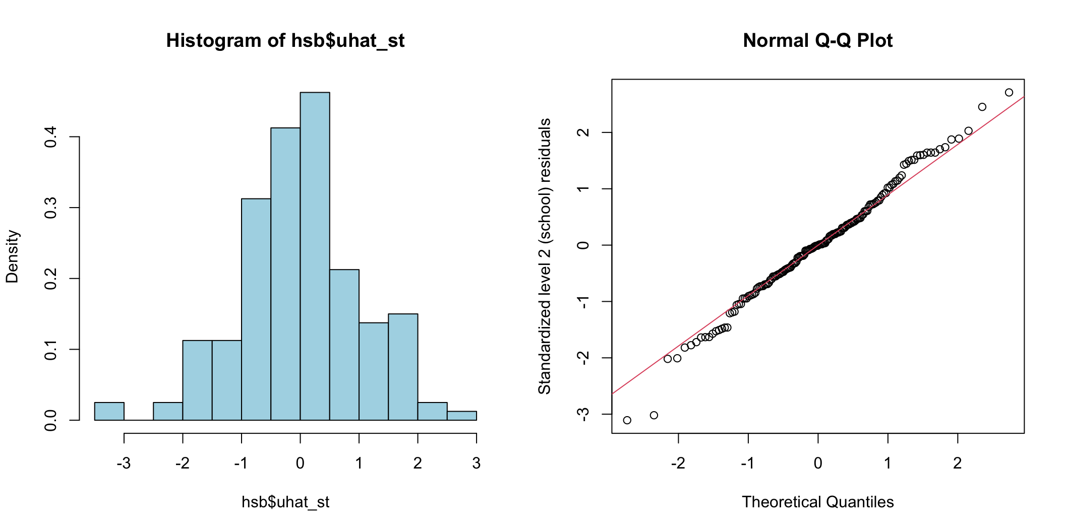
圖 74.4: Histogram and Q-Q plot of cluster (school) level standardized residuals for the intercept
par(mfrow=c(1,2))
hist(hsb_selected$ehat, freq = FALSE, breaks = 38, col='lightblue')
qqnorm(hsb_selected$ehat,  ylab = "Standardized level 1 (pupil) residuals"); qqline(hsb_selected$ehat, col=2)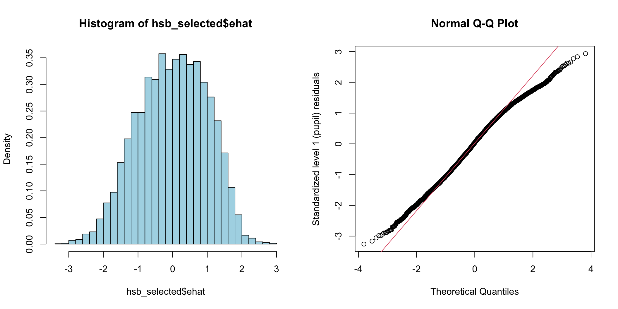
圖 74.5: Histogram and Q-Q plot of individual (pupil) level standardized residuals for the intercept
74.8.10 通過剛剛所求的隨機效應方差的殘差,確認哪個學校存在相對極端的值。
# summ(hsb$uhat_st, graph = FALSE)
hsb %>%
  summarise(n = n(),
            mean_uhatst = mean(uhat_st),
            sd_uhatst = sd(uhat_st),
            min_uhatst = min(uhat_st),
            max_uhatst = max(uhat_st))
## n mean_uhatst sd_uhatst min_uhatst max_uhatst
## 1 160 -0.00078526873 1.0066282 -3.1071846 2.7097312## sector mathach size uhat_st
## 48 1 13.874 687 2.7097312## sector mathach size uhat_st
## 135 0 15.9359999 153 -3.0189027
## 143 0 -2.0810001 745 -3.1071846所以,此處可以看出,隨機效應殘差下提示的隨機效應標準差可能比較極端的有上面這三所規模較小的學校。其中一所是天主教會學校,另外兩所是非天主教會學校。
74.8.11 計算學校水平的 SES 平均值,以及每個學生自己和所在學校均值之間的差值大小。分別擬合兩個不同的混合效應模型,一個只用 SES,另一個換做使用新計算的組均值和組內均差。
Mean_ses_math <- ddply(hsb_selected,~schoolid,summarise,mean_ses=mean(ses),mean_math=mean(mathach))


hsb_selected$dif_ses <- NA
for (i in Mean_ses_math$schoolid) {
hsb_selected$dif_ses[which(hsb_selected$schoolid == i)] <-  hsb_selected$ses[which(hsb_selected$schoolid == i)] -
  Mean_ses_math$mean_ses[which(Mean_ses_math$schoolid == i)]
}

hsb_selected <- hsb_selected %>%
  mutate(mean_ses = ses - dif_ses)

## total simple model with ses only
Simple_reml <- lmer(mathach ~ ses + (1 | schoolid), data = hsb_selected, REML = TRUE)
summary(Simple_reml)
## Linear mixed model fit by REML. t-tests use Satterthwaite's method ['lmerModLmerTest']
## Formula: mathach ~ ses + (1 | schoolid)
## Data: hsb_selected
##
## REML criterion at convergence: 46645.2
##
## Scaled residuals:
## Min 1Q Median 3Q Max
## -3.126073 -0.727203 0.021883 0.757717 2.919116
##
## Random effects:
## Groups Name Variance Std.Dev.
## schoolid (Intercept) 4.7682 2.1836
## Residual 37.0344 6.0856
## Number of obs: 7185, groups: schoolid, 160
##
## Fixed effects:
## Estimate Std. Error df t value Pr(>|t|)
## (Intercept) 12.65748 0.18799 148.30225 67.332 < 2.2e-16 ***
## ses 2.39020 0.10572 6838.07757 22.609 < 2.2e-16 ***
## ---
## Signif. codes: 0 '***' 0.001 '**' 0.01 '*' 0.05 '.' 0.1 ' ' 1
##
## Correlation of Fixed Effects:
## (Intr)
## ses 0.003## fit the extended model within and between effect separated
Extend_reml <- lmer(mathach ~ dif_ses + mean_ses + (1 | schoolid), data = hsb_selected, REML = TRUE)
## the between schools effect (5.87) seems much larger than the within school effect (2.19)
summary(Extend_reml)## Linear mixed model fit by REML. t-tests use Satterthwaite's method ['lmerModLmerTest']
## Formula: mathach ~ dif_ses + mean_ses + (1 | schoolid)
## Data: hsb_selected
##
## REML criterion at convergence: 46568.6
##
## Scaled residuals:
## Min 1Q Median 3Q Max
## -3.16665 -0.72543 0.01744 0.75578 2.94540
##
## Random effects:
## Groups Name Variance Std.Dev.
## schoolid (Intercept) 2.6925 1.6409
## Residual 37.0191 6.0843
## Number of obs: 7185, groups: schoolid, 160
##
## Fixed effects:
## Estimate Std. Error df t value Pr(>|t|)
## (Intercept) 12.68331 0.14938 153.65182 84.906 < 2.2e-16 ***
## dif_ses 2.19117 0.10867 7021.50918 20.164 < 2.2e-16 ***
## mean_ses 5.86617 0.36170 153.36659 16.218 < 2.2e-16 ***
## ---
## Signif. codes: 0 '***' 0.001 '**' 0.01 '*' 0.05 '.' 0.1 ' ' 1
##
## Correlation of Fixed Effects:
## (Intr) dif_ss
## dif_ses 0.000
## mean_ses 0.010 0.000## We find strong evidence to support that the second model gives a better fit to the data
mod2<- update(Extend_reml, . ~ . - dif_ses - mean_ses)
anova(Extend_reml, mod2)## refitting model(s) with ML (instead of REML)## Data: hsb_selected
## Models:
## mod2: mathach ~ (1 | schoolid)
## Extend_reml: mathach ~ dif_ses + mean_ses + (1 | schoolid)
## npar AIC BIC logLik deviance Chisq Df Pr(>Chisq)
## mod2 3 47121.8 47142.4 -23557.9 47115.8
## Extend_reml 5 46573.8 46608.2 -23281.9 46563.8 552.001 2 < 2.22e-16 ***
## ---
## Signif. codes: 0 '***' 0.001 '**' 0.01 '*' 0.05 '.' 0.1 ' ' 1