第 47 章 直線和曲線 curves and lines
兩種方式,一種是多項式回歸模型 (polynomial regression),另一種是 B-spline。
47.1 多項式回歸模型
使用二次,三次或者多次項構建預測變量的結構。
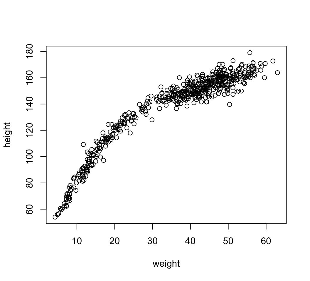
圖 47.1: The relationship is visibly curved, because we have included the non-adult individuals.
顯然我們有理由考慮使用二次方程的拋物線形式來做這個數據的模型:
\[ \mu_i = \alpha + \beta_1 x_i + \beta_2 x_i^2 \]
其完整的模型可以描述為:
\[ \begin{aligned} h_i & \sim \text{Normal}(\mu_u, \sigma) \\ \mu_i & = \alpha + \beta_1 x_i + \beta_2 x_i^2 \\ \alpha & \sim \text{Normal}(178, 20) \\ \beta_1 & \sim \text{Log-normal}(0, 1) \\ \beta_2 & \sim \text{Normal}(0, 1) \\ \sigma & \sim \text{Uniform}(0, 50) \end{aligned} \]
d$weight_s <- (d$weight - mean(d$weight)) / sd(d$weight)
d$weight_s2 <- d$weight_s^2

m4.5 <- quap(
  alist(
    height ~ dnorm( mu, sigma),
    mu <- a + b1*weight_s + b2*weight_s2,
    a ~ dnorm( 178, 20 ),
    b1 ~ dlnorm( 0, 1 ),
    b2 ~ dnorm( 0, 1 ),
    sigma ~ dunif(0 , 50)
  ),  data = d
)


precis(m4.5)
## mean sd 5.5% 94.5%
## a 146.0574158 0.36897479 145.4677228 146.6471088
## b1 21.7330542 0.28888840 21.2713548 22.1947537
## b2 -7.8032786 0.27418323 -8.2414764 -7.3650809
## sigma 5.7744619 0.17646418 5.4924380 6.0564857weight.seq <- seq( from = -2.2, to = 2, length.out = 30)
pred_dat <- list(weight_s = weight.seq, weight_s2 = weight.seq^2)
mu <- link( m4.5, data = pred_dat)
mu.mean <- apply(mu, 2, mean)
mu.PI <- apply( mu, 2, PI, prob = 0.89)
sim.height <- sim( m4.5, data = pred_dat)
height.PI <- apply( sim.height, 2, PI, prob = 0.89)plot( height ~ weight_s, d, col = col.alpha(rangi2, 0.5))
lines( weight.seq, mu.mean )
shade( mu.PI, weight.seq)
shade(height.PI, weight.seq)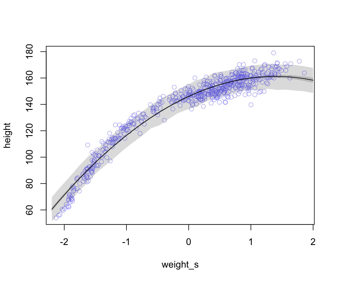
圖 47.2: Polynomial (a second order, quadratic) regressions of height on weight (standardized) for the height data. The solid curves show the path of mu in the model, and the shaded regions show the 89% interval of the mean (close to the solid curve), and the 89% interval of predictions (wider).
你可以更進一步,使用一個三次方(cubic)模型來看看是否接近實際數據本身的分佈。
\[ \begin{aligned} h_i & \sim \text{Normal}(\mu_u, \sigma) \\ \mu_i & = \alpha + \beta_1 x_i + \beta_2 x_i^2 + \beta_3x_i^3\\ \alpha & \sim \text{Normal}(178, 20) \\ \beta_1 & \sim \text{Log-normal}(0, 1) \\ \beta_2 & \sim \text{Normal}(0, 1) \\ \beta_3 & \sim \text{Normal}(0, 1) \\ \sigma & \sim \text{Uniform}(0, 50) \end{aligned} \]
d$weight_s3 <- d$weight_s^3
m4.6 <- quap(
alist(
height ~ dnorm( mu, sigma),
mu <- a + b1*weight_s + b2*weight_s2 + b3*weight_s3,
a ~ dnorm( 178, 20 ),
b1 ~ dlnorm( 0, 1 ),
b2 ~ dnorm( 0, 1 ),
b3 ~ dnorm( 0, 1 ),
sigma ~ dunif(0 , 50)
), data = d
)
precis(m4.6)## mean sd 5.5% 94.5%
## a 146.3945405 0.30998713 145.8991212 146.8899598
## b1 15.2197281 0.47626526 14.4585642 15.9808920
## b2 -6.2026117 0.25715822 -6.6136002 -5.7916232
## b3 3.5833790 0.22877341 3.2177549 3.9490031
## sigma 4.8298893 0.14694262 4.5950466 5.0647320weight.seq <- seq( from = -2.2, to = 2, length.out = 30)
pred_dat <- list(weight_s = weight.seq,
weight_s2 = weight.seq^2,
weight_s3 = weight.seq^3)
mu <- link( m4.6, data = pred_dat)
mu.mean <- apply(mu, 2, mean)
mu.PI <- apply( mu, 2, PI, prob = 0.89)
sim.height <- sim( m4.6, data = pred_dat)
height.PI <- apply( sim.height, 2, PI, prob = 0.89)
plot( height ~ weight_s, d, col = col.alpha(rangi2, 0.5))
lines( weight.seq, mu.mean )
shade( mu.PI, weight.seq)
shade(height.PI, weight.seq)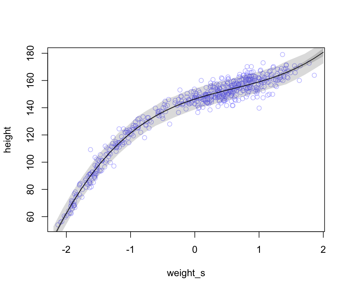
圖 47.3: Polynomial (a third order, cubic) regressions of height on weight (standardized) for the height data. The solid curves show the path of mu in the model, and the shaded regions show the 89% interval of the mean (close to the solid curve), and the 89% interval of predictions (wider).
在使用標準化的 Z 值計算之後,如果你希望恢復到原來的尺度,而不是標準化的 x 軸,可以按照以下步驟:
plot( height ~ weight_s, d, col = col.alpha(rangi2, 0.50), xaxt = "n")
at <- c(-2, -1, 0, 1, 2)
labels <- at*sd(d$weight) + mean(d$weight)
axis( side = 1, at = at, labels = round(labels, 1))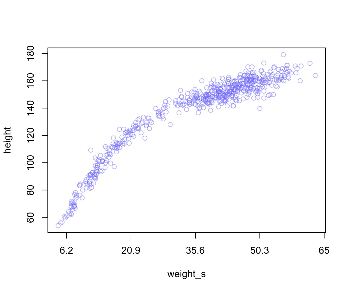
圖 47.4: Converting back to natural scale.
47.2 平滑曲線 Splines
B-Splines 是基礎 (basic) 平滑曲線的涵義。下面的數據紀錄了每年春天櫻花開放的日期:
##                    mean           sd      5.5%      94.5%       histogram
## year       1408.0000000 350.88459641 867.77000 1948.23000   ▇▇▇▇▇▇▇▇▇▇▇▇▁
## doy         104.5405079   6.40703618  94.43000  115.00000        ▁▂▅▇▇▃▁▁
## temp          6.1418861   0.66364787   5.15000    7.29470        ▁▃▅▇▃▂▁▁
## temp_upper    7.1851512   0.99292057   5.89765    8.90235 ▁▂▅▇▇▅▂▂▁▁▁▁▁▁▁
## temp_lower    5.0989413   0.85034959   3.78765    6.37000 ▁▁▁▁▁▁▁▃▅▇▃▂▁▁▁
其中每年第一次確認的開花的日期被紀錄為 doy 變量。它的範圍是在每年的第 86 (三月底) ~124 (五月初)天:
## [1] 86 124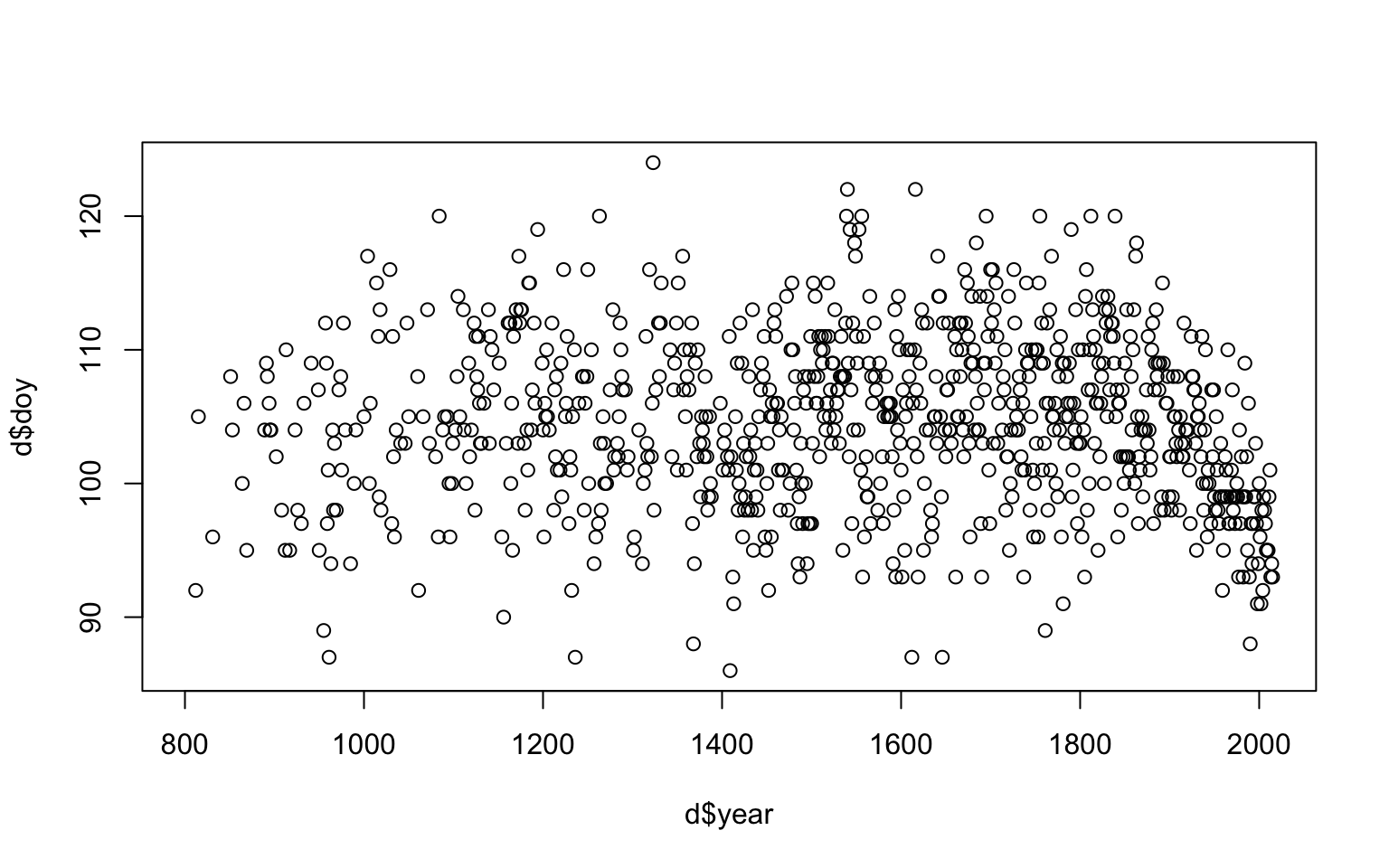
圖 47.5: 橫軸是年份,縱軸是每年第一天開花的日子
為了評估這個每年第一天開花紀錄的日期是否隨著時間有怎樣的變化趨勢,我們選擇使用基礎平滑曲線的方法:
\[ \mu_i = \alpha + w_1 B_{i,1} + w_2 B_{i,2} + w_3 B_{i,3} + \dots \]
其中,
- \(B_{i,n}\) 是橫軸第 \(i\) 年份的第 \(n\) 個區間的基礎函數 (basis function)
- \(w_n\) 是該基礎函數本身的權重
假定我們選擇使用 15 個節點 (knots),也就是 \(n = 15\),來繪製該數據的平滑曲線:
d2 <- d[complete.cases(d$doy), ] # complete cases on doy
num_knots <- 15
knot_list <- quantile( d2$year, probs = seq(0, 1, length.out = num_knots))

str(knot_list)
## Named num [1:15] 812 1036 1174 1269 1377 ...
## - attr(*, "names")= chr [1:15] "0%" "7.142857%" "14.28571%" "21.42857%" ...## 0% 7.142857% 14.28571% 21.42857% 28.57143% 35.71429% 42.85714% 50% 57.14286% 64.28571%
## 812 1036 1174 1269 1377 1454 1518 1583 1650 1714
## 71.42857% 78.57143% 85.71429% 92.85714% 100%
## 1774 1833 1893 1956 2015我們來建立一個三次方平滑曲線,cubic spline:
##               1           2             3             4 5 6 7 8 9 10 11 12 13 14 15 16 17
## [1,] 1.00000000 0.000000000 0.00000000000 0.0000000e+00 0 0 0 0 0  0  0  0  0  0  0  0  0
## [2,] 0.96035713 0.039312303 0.00032983669 7.2860303e-07 0 0 0 0 0  0  0  0  0  0  0  0  0
## [3,] 0.76650948 0.220745951 0.01255948103 1.8509216e-04 0 0 0 0 0  0  0  0  0  0  0  0  0
## [4,] 0.56334070 0.385673722 0.04938483524 1.6007409e-03 0 0 0 0 0  0  0  0  0  0  0  0  0
## [5,] 0.54526700 0.398683678 0.05418946879 1.8598537e-03 0 0 0 0 0  0  0  0  0  0  0  0  0
## [6,] 0.45273210 0.459759692 0.08371386242 3.7943487e-03 0 0 0 0 0  0  0  0  0  0  0  0  0
B 其實是一個 827 行,17 列的矩陣。每一行是一個年份,對應 d2 數據框的每一行。每一列,則是對應一個基礎函數 basic function。為了繪製這些基礎函數,我們可以把他們和對應的年份作圖:
plot(NULL, xlim = range(d2$year), ylim = c(0, 1),
     xlab = "year", ylab = "basis")
for( i in 1:ncol(B)) lines( d2$year, B[, i])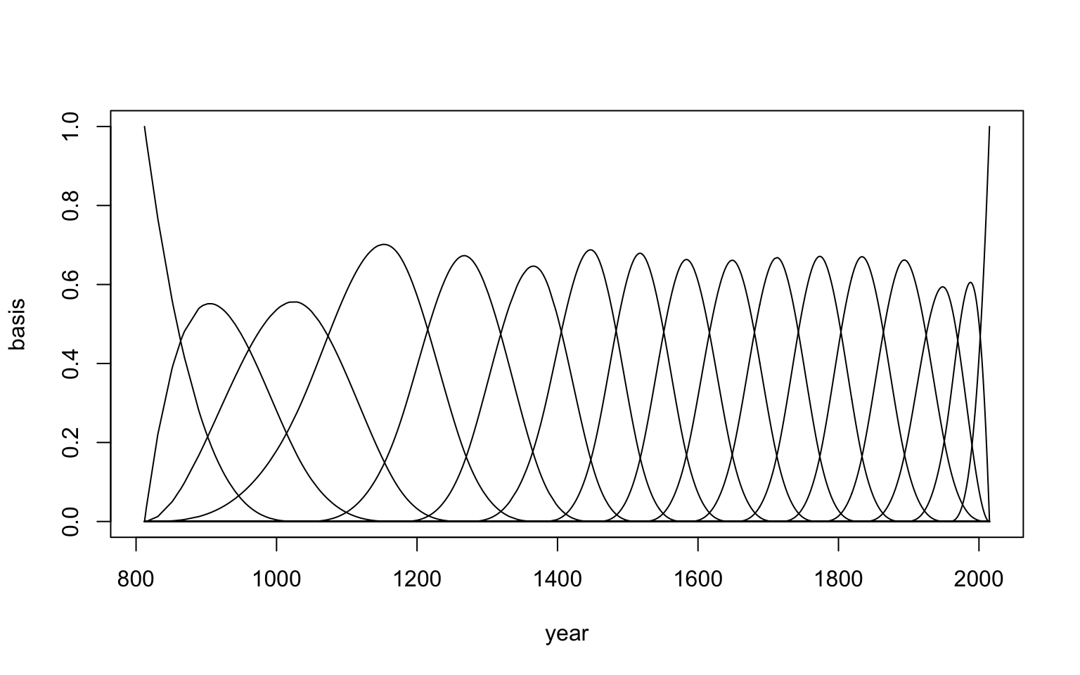
圖 47.6: the basic functions of the blossom data with 15 knots.
模型本身只是一個簡單線型回歸其實:
\[ \begin{aligned} D_i & \sim \text{Normal}(\mu_i, \sigma) \\ \mu_i & = \alpha + \sum_{k = 1}^K w_k B_{k,i} \\ \text{Priors :} & \\ \alpha & \sim \text{Normal}(100, 10) \\ w_j & \sim \text{Normal}(0, 10) \\ \sigma & \sim \text{Exponential} (1) \end{aligned} \] 對於像方差,標準差這樣必須大於零的參數來說,選用指數分佈作為先驗概率分佈其實是比較常見的。
實際運算這個模型,獲取 \(w_j\) 們的事後概率分佈:
m4.7 <- quap(
  alist(
    D ~ dnorm( mu, sigma ),
    mu <- a + B %*% w ,
    a ~ dnorm(100, 10),
    w ~ dnorm(0, 10),
    sigma ~ dexp(1)
  ), data = list(D = d2$doy, B = B),
  start = list( w = rep(0, ncol(B)))
)

precis(m4.7, depth = 2)
## mean sd 5.5% 94.5%
## w[1] -3.01975939 3.86116673 -9.190649574 3.15113078
## w[2] -0.83435191 3.87014567 -7.019592169 5.35088835
## w[3] -1.05229324 3.58491642 -6.781682058 4.67709559
## w[4] 4.84212482 2.87708709 0.243983966 9.44026566
## w[5] -0.83877820 2.87429504 -5.432456817 3.75490041
## w[6] 4.32684717 2.91481867 -0.331596025 8.98529036
## w[7] -5.32336368 2.80017706 -9.798587450 -0.84813991
## w[8] 7.84857262 2.80203636 3.370377332 12.32676792
## w[9] -1.00540484 2.88100207 -5.609802577 3.59899290
## w[10] 3.03456155 2.91006945 -1.616291474 7.68541458
## w[11] 4.67146784 2.89167834 0.050007362 9.29292832
## w[12] -0.15856869 2.86936616 -4.744370007 4.42723262
## w[13] 5.56832971 2.88738944 0.953723710 10.18293571
## w[14] 0.70828833 2.99925702 -4.085103668 5.50168033
## w[15] -0.79633311 3.29347388 -6.059940468 4.46727424
## w[16] -6.96872059 3.37571746 -12.363769079 -1.57367209
## w[17] -7.66032665 3.22272168 -12.810858321 -2.50979497
## a 103.34854121 2.36968067 99.561333816 107.13574861
## sigma 5.87661606 0.14375338 5.646870395 6.10636172繪製增加了權重 \(w_j\) 和基礎函數結合的平滑曲線:
post <- extract.samples( m4.7 )
w <- apply( post$w, 2, mean )

plot(NULL, xlim = range(d2$year), ylim = c(-6, 6),
     xlab = "year", ylab = "basis * weight")
for( i in 1 : ncol(B)) lines( d2$year, w[i]*B[,i])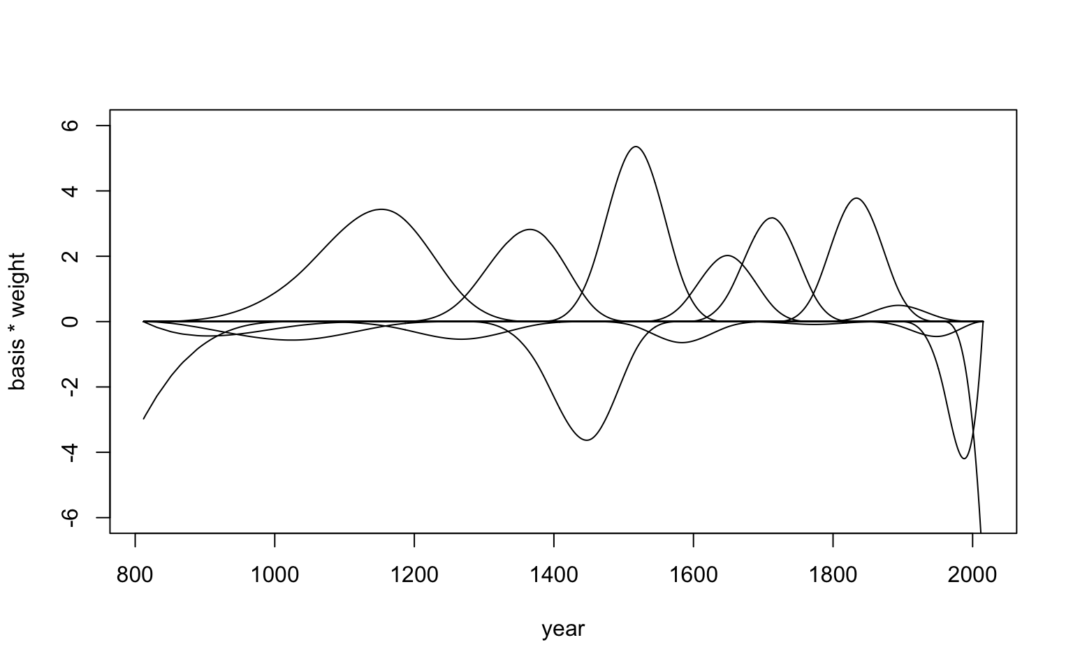
圖 47.7: The cubic spline of the blossom data with 15 knots. (each basis weighted by its correponding parameter)
## [1] 1000 827## [1] 2 827mu_mean <- apply( mu, 2, mean)
plot( d2$year, d2$doy, col = col.alpha(rangi2, 0.3), pch = 16)
lines(d2$year, mu_mean)
shade(mu_PI, d2$year, col = col.alpha("black", 0.5))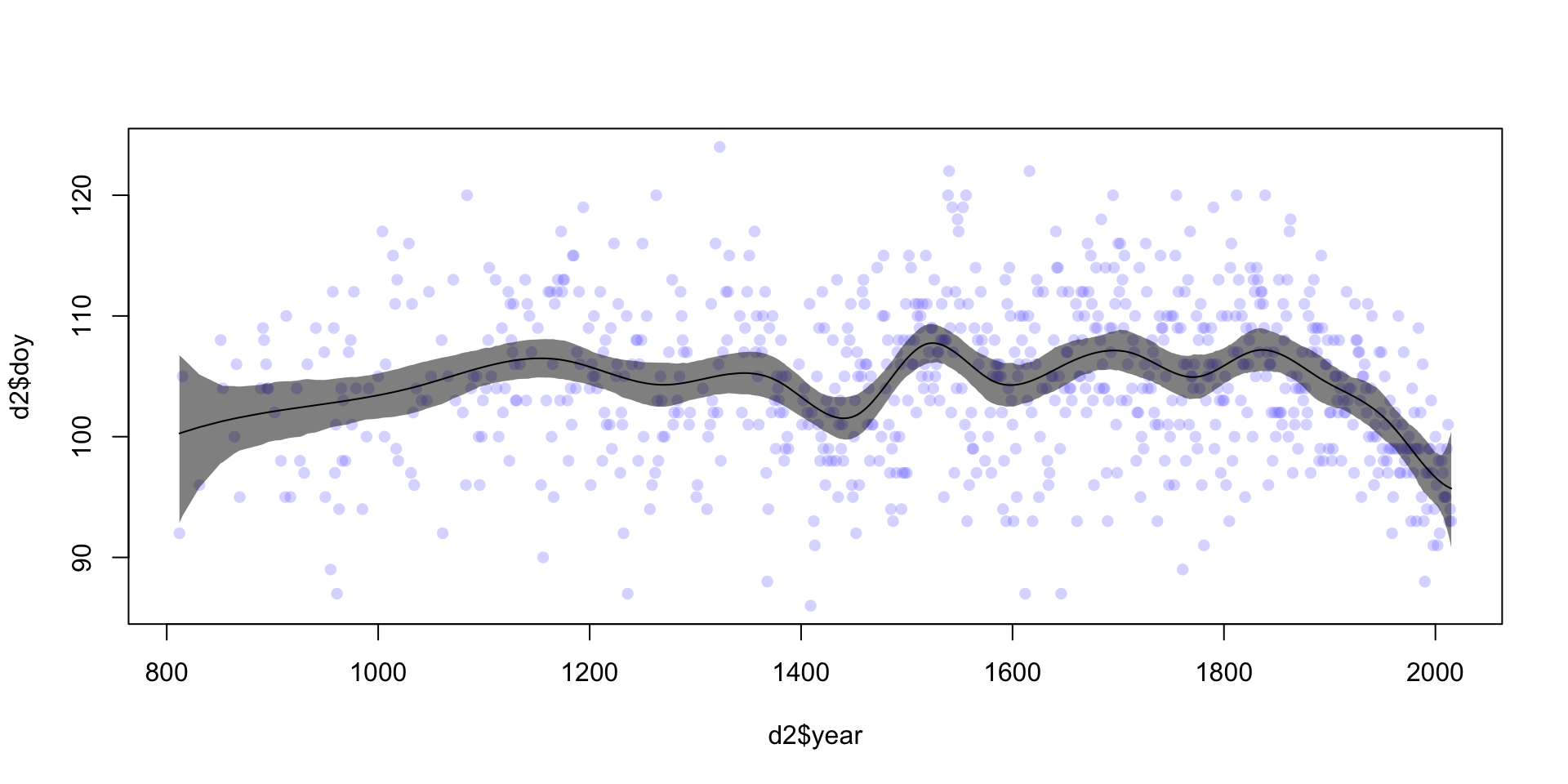
圖 47.8: The cubic spline of the blossom data with 15 knots. (the sum of these weighted basis functions, at each point, produces the spline. displayed as 97% posterior interval of mu.)
圖形顯示的開花時間和年份之間的曲線關係,可見在1500年前後發生了某些情況。而且近年來似乎有提早開花的傾向。