第 42 章 貝葉斯定理的應用:單一參數模型 Single-parameter models
從前一章節我們可以深切體會到,貝葉斯統計是如何讓我們的先驗概率,在觀察到數據之後,更新信息,獲得事後概率 (這是一個通過數據自我學習,進化的過程)。(How a prior belief about an event can be updated, given data, to a posterior belief.)
所以說,在貝葉斯模型中,我們期待使用觀察數據來學習,以增加現有的對相關參數的知識和信息。本章我們把重點放在二項分佈,用二項分佈作爲單一參數模型來瞭解怎樣推導事後分佈。
42.1 從二進制數據中估計概率 Estimating a probability from binomial data
在簡單的二項分佈模型中,我們討論的目的是希望從一系列的“柏努利試驗 Bernoulli trials”的結果來估計一個未知的總體百分比 (unknown population proportion)。既 \(y_1, y_2, \dots, y_n\) 的結果是 \(0,1\)。所以二項分佈的採樣模型可以寫作是:
\[ p(y | \theta) = \text{Bin}(y | n, \theta) = {n \choose y}\theta^y(1- \theta)^{n -y} \]
Example 42.1 估計新生兒中女嬰的比例。
作為二項分佈模型最典型的應用之一,估計新生兒中男女性別的比例,也就是男嬰或者女嬰的百分比估計是長期以來茶餘飯後的話題之一。二百年前,歐洲人群中就有好事者估計過,新生兒中女嬰的比例應該是小於50%的。現在大家更加關心的其實是,有哪些因素可能會影響新生兒中女嬰的比例。如今,大多數科學界認可的歐洲人口中新生兒女嬰的比例是 0.485。
在這個例子中,我們定義
- 這個未知的新生兒女嬰比例是 \(\theta\)。當然可能有人不同意,或者更樂意使用男女新生兒人數比例 \(\phi = \frac{(1 - \theta)}{\theta}\),來描述這個問題,這個大同小異。
- \(y\) 是新生兒中女嬰的人數。
- \(n\) 是新生兒總人數。
當我們決定使用二項分佈模型來模擬上述情境的數據時,我們默認了新生兒性別比例這一條件是決定性別的唯一條件,也就是說,除了這個 \(\theta\) 之外,性別是完全隨機且互相獨立的(此處需要先忽略掉一胞多胎,和同一家庭因素等可能對新生兒性別造成的影響)。那麼應用了貝葉斯定理之後,我們可以推導獲得 \(\theta\) 的事後概率分佈是
\[ \begin{equation} p(\theta | y) \propto \theta^y (1 - \theta)^{n - y} \end{equation} \tag{42.1} \]
由於 \(n,y\) 都是常數項,僅由他們構成的最前面的部分就是一個不會根據 \(\theta\) 取值發生改變的部分,所以在計算事後概率分佈的事後,我們可以把這部分忽略掉,使用它的非。根據 Beta 分佈的性質,不難發現,公式 (42.1) 其實就是一個參數為 \(y + 1, n - y + 1\) 的 Beta 分佈:
\[ \begin{equation} \theta | y \sim \text{Beta}(y + 1, n - y + 1) \end{equation} \tag{42.2} \]
42.1.1 事後概率分佈是數據和先驗概率分佈之間的妥協
貝葉斯推斷的過程是從先驗概率分佈 \(p(\theta)\) 過渡到事後概率分佈 \(p(\theta | y)\) 的過程。我們應該會很自然地認為,這先驗和事後之間的概率分佈必然存在這某種聯繫。例如,我們可能會很純粹的認為,因為事後概率分佈增加了手上數據的信息,那麼它相應地應該比先驗概率分佈不那麼分散(less variable than the prior)。這個思考過程可以通過下面的數學關係來呈現:
- \(\theta\) 的事後概率分佈的期望 \(E(\theta | y)\) 和它的先驗概率分佈的期望 \(E(\theta)\) 之間的關係:
\[ \begin{equation} E(\theta) = E(E(\theta | y)) \end{equation} \tag{42.3} \] 事後概率分佈的期望 公式(42.3) 很好理解。先驗概率分佈的 \(\theta\) 均值 \(E(\theta)\),等於事後概率分佈的 \(\theta\),在所有觀察點 \(y\) 時的值的平均值。
- \(\theta\) 的事後概率分佈的方差 \(\text{var}(\theta | y)\) 和先驗概率分佈方差之間的關係
\[ \begin{equation} \text{var}(\theta) = E(\text{var}(\theta | y)) + \text{var}(E(\theta | y)) \end{equation} \tag{42.4} \]
方差關係的方程式 (42.4) 其實說的是先驗概率分佈的方差,在獲取了新的數據 \(y\) 之後被分成了兩部分。一個是事後概率分佈本身的方差的均值 \(E(\text{var}(\theta | y))\),還有一部分是事後概率分佈均值的方差 \(\text{var}(E(\theta | y))\)。
證明方差關係的公式 (42.4) 參考概率論部分期望與方差的關係 (Chapter 3)
\[ \begin{aligned} E(\text{var}(\theta | y)) + \text{var}(E(\theta | y)) & = E(E(\theta^2 | y) - (E(\theta | y))^2) + E([E(\theta | y)]^2) - [E(E(\theta | y))]^2 \\ & = E(\theta^2) - E([E(\theta | y)]^2) + E([E(\theta | y)]^2) - [E(\theta)]^2 \\ & = E(\theta^2) - [E(\theta)]^2 \\ & = \text{var}(\theta) \end{aligned} \]
理解了上述關係之後,可以說,事後概率分佈的方差總是比先驗概率分佈的方差要小一些。如果能想方設法使事後概率分佈均值的方差 \(\text{var}(E(\theta | y))\) 這部分佔據更大部分,我們就能提高對 \(\theta\) 的事後估計精確度。(the greater the latter variation, the more the potential for reducing our uncertainty with regard to \(\theta\)).
這也是貝葉斯統計推斷的基本特徵之一,事後概率分佈的中心,一般是位於先驗概率分佈的中心,和觀察數據的中心之間的某個地方,它是先驗概率分佈和數據之間相互妥協的結果。
Example 42.2 估計有前置胎盤的母親生下的新生兒中女嬰的比例。
一個早期來自德國的研究觀察到,980 名孕期有前置胎盤的母親生下的新生兒中,有 437 名是女嬰。那麼,如何來比較這個觀察數據和已知的,在總體人群 (general population) 中的女嬰出生比例 0.485之間的差異?
當先驗概率分佈使用均一分佈 (uniform distribution: \(\theta \sim \text{Beta}(a = 1, b = 1)\)) 時,我們獲得的數據是 \(n = 980, y = 437\)。那麼根據共軛的性質可以計算出事後概率分佈是服從另一個 Beta 分佈: \(p(\theta | y,n) = \text{Beta}(a + y, b + n - y) = \text{Beta}(438, 544)\)
# 95% Credible Intervals
L <- qbeta(0.025, 438, 544)
U <- qbeta(0.975, 438, 544)

post <- Vectorize(function(theta) dbeta(theta, 438, 544))

# Illustration
x1 <- seq(0.375, 0.525,length=10000)
y1 <- post(x1)
plot(x1, y1, type = "l", xlab=~theta, ylab="Density",
     main = "Uniform prior -> Posterior is Beta(438, 544)",
     lwd = 2, frame.plot = FALSE)
abline(v = 0.488, col = "blue", lty = 3, lwd = 2)

polygon(c(L, x1[x1>=L & x1<= U], U), c(0, y1[x1>=L & x1<=U], 0), col="lightblue")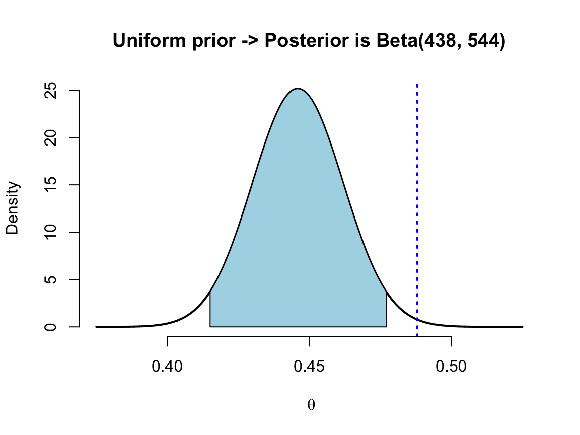
圖 42.1: Probability of a girl given placenta previa (BDA3, p.37).
使用 ggplot2 繪圖的方法如下,參考原作者的代碼
# seq creates evenly spaced values
df1 <- data.frame(theta = seq(0.375, 0.525, 0.001))
a <- 438
b <- 544
# dbeta computes the posterior density
df1$p <- dbeta(df1$theta, a, b)

## 計算95%可信區間
# seq creates evenly spaced values from 2.5% quantile
# to 97.5% quantile (i.e., 95% central interval)
# qbeta computes the value for a given quantile given parameters a and b
df2 <- data.frame(theta = seq(qbeta(0.025, a, b), qbeta(0.975, a, b), length.out = 100))
# compute the posterior density
df2$p <- dbeta(df2$theta, a, b)


ggplot(mapping = aes(theta, p)) +
  geom_line(data = df1) +
  # Add a layer of colorized 95% posterior interval
  geom_area(data = df2, aes(fill='1')) +
  # Add the proportion of girl babies in general population
  geom_vline(xintercept = 0.488, linetype='dotted') +
  # Decorate the plot a little
  labs(title='Uniform prior -> Posterior is Beta(438,544)', y = '') +
  scale_y_continuous(expand = c(0, 0.1), breaks = NULL) +
  scale_fill_manual(values = 'lightblue', labels = '95% posterior interval') +
  theme(legend.position = 'bottom', legend.title = element_blank())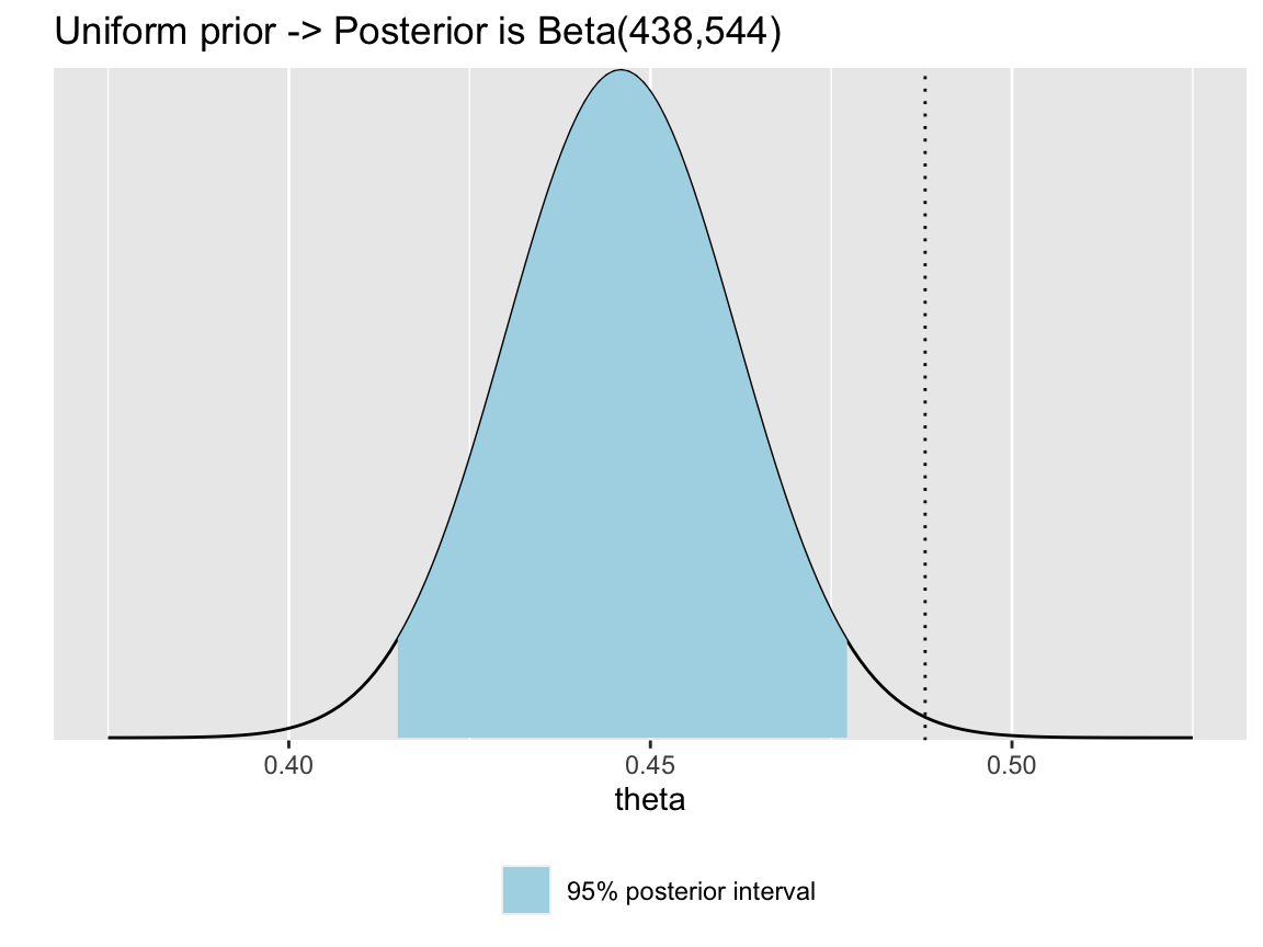
圖 42.2: Probability of a girl given placenta previa (BDA3, p.37), same figure in ggplot format.
可以看到這裡我們計算獲得的事後可信區間是 [0.415, 0.477],它的上限也低於總體人群的女嬰出生概率= 0.485。所以,應該可以認為如果有孕期有前置胎盤,女嬰出生的概率比人群水平更低。
## [1] 0.41506549## [1] 0.4771997742.1.2 不同先驗概率分佈對事後概率分佈估計的影響
參考原作者代碼
# Observed data: 437 girls and 543 boys
a <- 437
b <- 543

# Evaluate densities at evenly spaced points between 0.375 and 0.525
df1 <- data.frame(theta = seq(0.375, 0.525, 0.001))

# Posterior with Beta(1,1), ie. uniform prior

df1$pu <- dbeta(df1$theta, a+1, b+1)

# 3 different choices for priors

# Beta(0.488*2,(1-0.488)*2)
# Beta(0.488*20,(1-0.488)*20)
# Beta(0.488*200,(1-0.488)*200)

n <- c(2, 20, 200) # prior counts
apr <- 0.488 # prior ratio of success


# helperf returns for given number of prior observations, prior ratio
# of successes, number of observed successes and failures and a data
# frame with values of theta, a new data frame with prior and posterior
# values evaluated at points theta.
helperf <- function(n, apr, a, b, df)
  cbind(df,
        pr = dbeta(df$theta, n*apr, n*(1-apr)),
        po = dbeta(df$theta, n*apr + a, n*(1-apr) + b),
        n = n)

# lapply function over prior counts n and gather results into key-value pairs.
df2 <- lapply(n, helperf, apr, a, b, df1) %>% # calculate posterior points
  do.call(rbind, args = .) %>% # combine lists
  gather(grp, p, -c(theta, n), factor_key = T)

# add correct labels for plotting
df2$title <- factor(paste0('alpha/(alpha+beta)=0.488, alpha+beta=',df2$n))
levels(df2$grp) <- c('Posterior with unif prior', 'Prior', 'Posterior')

# Plot distributions

ggplot(data = df2) +
  geom_line(aes(theta, p, color = grp)) +
  geom_vline(xintercept = 0.488, linetype = 'dotted') +
  facet_wrap(~title, ncol = 1) +
  labs(x = '', y = '') +
  scale_y_continuous(breaks = NULL) +
  theme(legend.position = 'bottom', legend.title = element_blank())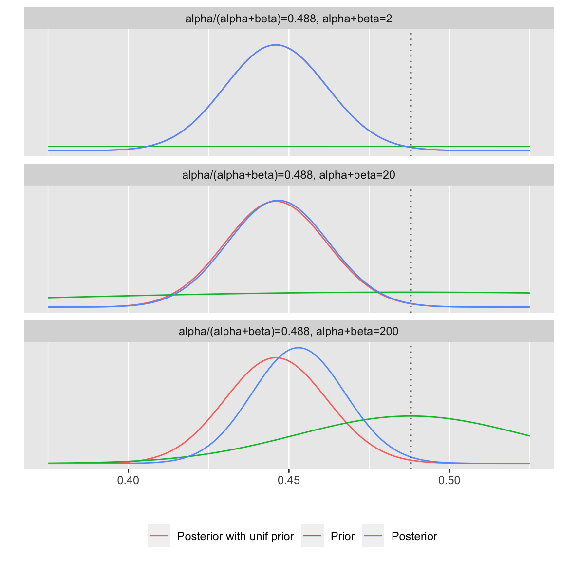
圖 42.3: Probability of a girl given placenta previa (BDA3, p.37), illustrate the effect of prior and compare posteriro distributions with different parameter values for the beta prior distribution.
不難觀察到,隨著先驗概率分佈的信息量增加(越往下的圖中先驗概率分佈的樣本量越多),事後概率分佈會被先驗概率分佈帶著往先驗概率的方向(也就是上圖中的右側)走,這始終顯示了事後概率分佈是先驗概率和數據本身相互妥協的結果。
42.1.3 從已知的事後概率分佈中採樣,對採集的事後樣本數據轉換
參考原作者代碼
# 我們從事後概率分佈 Beta(438, 544) 中採集事後樣本,存儲到向量 `theta` 中
a <- 438
b <- 544

theta <- rbeta(10000, a, b)

# 計算每一個採集樣本的比值比 odds ratio

phi <- (1 - theta) / theta

# 計算事後概率分佈樣本,及其轉換之後的比值比的的 2.5% 和 97.5% 位點估計

quantiles <- c(0.025, 0.975)
thetaq <- quantile(theta, quantiles)
phiq <- quantile(phi, quantiles)

# 繪製事後樣本(及轉換的比值比)的 histogram

# merge the data into one data frame for plotting
df1 <- data.frame(phi,theta) %>% gather()
# merge quantiles into one data frame for plotting
df2 <- data.frame(phi = phiq, theta = thetaq) %>% gather()

ggplot() +
  geom_histogram(data = df1, aes(value), bins = 30) +
  geom_vline(data = df2, aes(xintercept = value), linetype = 'dotted') +
  facet_wrap(~key, ncol = 1, scales = 'free_x')  +
  labs(x = '', y = '') +
  scale_y_continuous(breaks = NULL)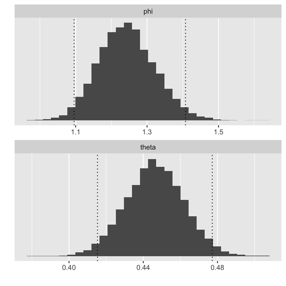
圖 42.4: Probability of a girl given placenta previa (BDA3, p.37), simulate samples from Beta(438, 544), draw a histogram with quantiles, and do the same for a transformed variable (the odds ratio).
42.1.4 使用非共軛先驗概率計算事後概率分佈
當使用非共軛先驗概率分佈時,事後概率分佈的計算就是直接用該非共軛先驗概率乘以數據的似然 (multiplying the non-conjugate prior and the likelihood at each data point)。從計算獲得的事後概率分佈中再採集樣本。
參考原作者的代碼。
# 觀察數據 (437, 543)

a <- 437
b <- 543

# 計算0.1~1之間相同間距(0.001)的事後概率密度(使用單一分佈Beta(1,1)作為先驗概率分佈)

df1 <- data.frame(theta = seq(0.1, 1, 0.001))
df1$con <- dbeta(df1$theta, a, b)

# 計算離散型非共軛先驗概率分佈的數據點上的概率密度

pp <- rep(1, nrow(df1))
pi <- sapply(c(0.388, 0.488, 0.588), function(pi) which(df1$theta == pi))
pm <- 11
pp[pi[1]:pi[2]] <- seq(1, pm, length.out = length(pi[1]:pi[2]))
pp[pi[3]:pi[2]] <- seq(1, pm, length.out = length(pi[3]:pi[2]))

# 除以概率密度總和 normalize the prior

df1$nc_p <- pp / sum(pp)

# 計算每個離散點上的非共軛事後概率分佈

po <- dbeta(df1$theta, a, b) * pp

# 除以事後概率分佈的總和 normalize the posterior

df1$nc_po <- po / sum(po)

# 繪製使用單一分佈後的事後概率,非共軛概率分佈本身,及其對應的非共軛事後概率分佈

# gather the data frame into key-value pairs
# and change variable names for plotting
df2 <- gather(df1, grp, p, -theta, factor_key = T)
levels(df2$grp) <- c('Posterior with uniform prior',
                     'Non-conjugate prior', 'Non-conjugate posterior')
ggplot(data = df2) +
  geom_line(aes(theta, p)) +
  facet_wrap(~grp, ncol = 1, scales = 'free_y') +
  coord_cartesian(xlim = c(0.35,0.6)) +
  scale_y_continuous(breaks=NULL) +
  labs(x = '', y = '')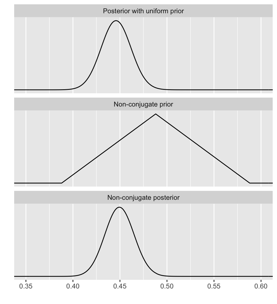
圖 42.5: Probability of a girl given placenta previa (BDA3, p.37). Calculate the posterior distribution on a discrete grid of points by multiplying the likelihood and a non-conjugate prior at each point, and normalizing over the points.
下面從非共軛事後概率分佈中採集樣本,使用逆累積密度函數 (inverse cdf sampling)
# 計算事後累積密度

df1$cs_po <- cumsum(df1$nc_po)

# 從單一分佈中採樣 Uniform(0, 1)
set.seed(2601)
# runif(k) returns k uniform random numbers from interval [0,1]
r <- runif(10000)

# 逆累積密度函數樣本採集 inverse-cdf sampling
# function to find the smallest value theta at which the cumulative
# sum of the posterior densities is greater than r.
invcdf <- function(r, df) df$theta[sum(df$cs_po < r) + 1]
# sapply function for each sample r. The returned values s are now
# random draws from the distribution.
s <- sapply(r, invcdf, df1)

# 繪製三個圖形 p1 是非共軛事後概率分佈;p2 是非共軛事後概率分佈的累積密度函數;p3 為從非共軛事後概率分佈中採集的樣本直方圖


p1 <- ggplot(data = df1) +
  geom_line(aes(theta, nc_po)) +
  coord_cartesian(xlim = c(0.35, 0.6)) +
  labs(title = 'Non-conjugate posterior', x = '', y = '') +
  scale_y_continuous(breaks = NULL)
p2 <- ggplot(data = df1) +
  geom_line(aes(theta, cs_po)) +
  coord_cartesian(xlim = c(0.35, 0.6)) +
  labs(title = 'Posterior-cdf', x = '', y = '') +
  scale_y_continuous(breaks = NULL)
p3 <- ggplot() +
  geom_histogram(aes(s), binwidth = 0.003) +
  coord_cartesian(xlim = c(0.35, 0.6)) +
  labs(title = 'Histogram of posterior samples', x = '', y = '') +
  scale_y_continuous(breaks = NULL)
# combine the plots
grid.arrange(p1, p2, p3)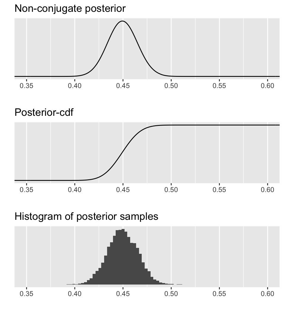
圖 42.6: Probability of a girl given placenta previa (BDA3, p.37). Simulate samples from the resulting non-standard posterior distribution using inverse cdf and the discrete grid.
42.2 貝葉斯理論下的事後二項分佈概率密度方程 notation for probability density functions in binomial data
- \(R\) 用來表示服從一個二項分佈的隨機變量, \(R\sim \text{Bin}(n, \theta)\)。
- \(r\) 表示觀察到 \(r\) 次成功實驗,實驗次數爲 \(n\)。
- 先驗概率分佈: \(\pi_\Theta(\theta)\)
- 應用貝葉斯定理:
\[ \begin{aligned} \pi_{\Theta|R}(\theta|r) &= \frac{f_R(r|\theta)\pi_\Theta(\theta)}{\int_0^1f_R(r|\theta)\pi_\Theta(\theta)\text{ d}\theta}\\ &= \frac{f_R(r|\theta)\pi_\Theta(\theta)}{f_R(r)} \end{aligned} \]
如果我們的先驗概率分佈:
\[\begin{equation} \pi_\Theta(\theta)=\begin{cases} 1 \text{ if } \theta=0.2\\ 0 \text{ otherwise} \end{cases} \end{equation}\]
意思就是,我們 100% 相信 \(\theta\) 絕對就等於 0.2,不相信 \(\theta\) 竟然還能取任何其他值(霸道自大又狂妄的我們)。
如果先驗概率分佈:
\[\begin{equation} \pi_\Theta(\theta)=\begin{cases} 0.4 \text{ if } \theta=0.2\\ 0.6 \text{ if } \theta=0.7 \end{cases} \end{equation}\]
意思就是,我們有 60% 的把握相信 \(\theta=0.7\),有 40% 的把握相信 \(\theta=0.2\),稍微傾向於 \(\theta=0.7\)。
假設進行10次實驗,觀察到3次成功。當 \(\theta=0.2\) 時,觀察數據的似然 (likelihood) 爲:
\[f_R(3|\theta=0.2)=\binom{10}{3}0.2^3(1-0.2)^7\]
當 \(\theta=0.7\) 時,觀察數據的似然爲:
\[f_R(3|\theta=0.7)=\binom{10}{3}0.7^3(1-0.7)^7\]
應用貝葉斯定理計算事後概率分佈:
\[ \begin{equation} \pi_{\Theta|R}(\theta|3)=\begin{cases} \frac{\binom{10}{3}0.2^3(1-0.2)^7\times0.4}{\binom{10}{3}0.2^3(1-0.2)^7\times0.4+\binom{10}{3}0.7^3(1-0.7)^7\times0.6}=0.937 \text{ if } \theta=0.2\\ \frac{\binom{10}{3}0.7^3(1-0.7)^7\times0.6}{\binom{10}{3}0.7^3(1-0.7)^7\times0.6+\binom{10}{3}0.2^3(1-0.2)^7\times0.4}=0.063 \text{ if }\theta=0.7 \end{cases} \end{equation} \]
所以,我們從一開始認爲只有40%的把握相信 \(\theta=0.2\),觀察數據告訴我們 10 次實驗,3次獲得了成功。所以我們現在有 93.7% 的把握相信 \(\theta=0.2\)。也就是說,觀察數據讓我們對參數 \(\theta\) 的取值可能性發生了質的變化,從原先的傾向於 \(\theta=0.7\) 到現在幾乎接近 100% 的認爲 \(\theta=0.2\)。也就是,觀察數據獲得的信息改變了我們的立場。
上面的例子很直觀,但是有下面幾個問題:
- 如果我們無法對參數 \(\theta\) 賦予先驗概率的點估計時,該怎麼辦?
- 如果事後概率不是一個離散的分佈時,該如何才能表達事後概率?
42.3 \(\theta\) 的先驗概率
一種選擇是,我們用均一分佈 (uniform distribution),即我們對數據一無所知,認爲所有的 \(\theta\) 的可能性都一樣,概率密度方程爲 \(1\)。在這一情況下,先驗概率爲 1: \(\pi_\Theta(\theta)=1\),其事後概率分佈爲:
\[ \begin{equation} \pi_{\Theta|R}(\theta|r)=\frac{\binom{n}{r}\theta^r(1-\theta)^{n-r}}{\int_0^1\binom{n}{r}\theta^r(1-\theta)^{n-r} \text{ d}\theta} \tag{42.5} \end{equation} \]
看到即使在如此簡單的先驗概率下,我們還是要使用複雜的微積分進行計算。幸運的是,像 (42.5) 的分母這樣的積分公式其實是有跡可循的。這就是 beta (\(\beta\)) 分佈。
42.3.1 beta 分佈 the beta distribution
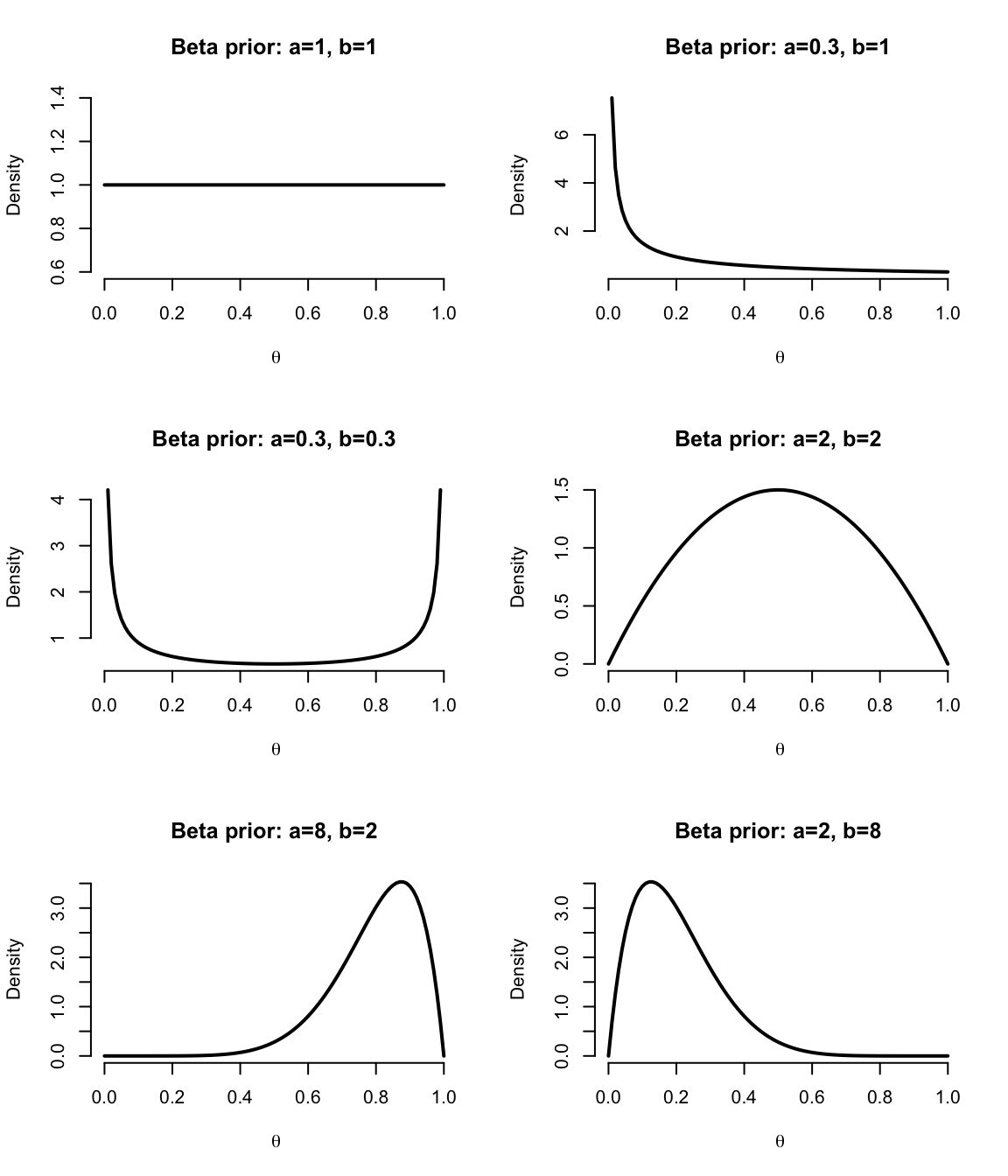
圖 42.7: Beta distribution functions for various values of a, b
你會發現,beta分佈的圖形特徵由它的兩個超參數 (hyperparameter) a, b 決定。當相對地 a 比較大的時候,beta分佈的概率多傾向於較靠近橫軸右邊,也就是1的位置(較高概率),相對地 b 比較大的時候,beta分佈的曲線多傾向於靠近橫軸左邊,也就是0的位置(較低概率)。如果 a 和 b同時都在變大的話,beta分佈的曲線就變得比較“瘦”。這樣決定概率分佈形狀的參數,又被叫做形狀參數 (shape parameters)
我們定義 \(a>0\) 時伽馬方程爲
\[\Gamma(a)=\int_0^\infty x^{a-1}e^{-ax}\text{ d}x\]
當 \(a\) 取正整數時, \(\Gamma(a)\) 是 \((a-1)!\)。例如,當 \(a=4, \Gamma(a)=3\times2\times1=6\)。
對於 \(\theta\in[0,1]\) 時,beta 方程 \(Beta(a,b)\) 被定義爲:
\[ \begin{aligned} \pi\Theta(\theta|a,b) &= \theta^{a-1}(1-\theta)^{b-1}\frac{\Gamma(a+b)}{\Gamma(a)\Gamma(b)}\\ &= \frac{\theta^{a-1}(1-\theta)^{b-1}}{B(a,b)} \end{aligned} \]
其中 \[B(a,b)=\frac{\Gamma(a)\Gamma(b)}{\Gamma(a+b)} = \int_0^1\theta^{a-1}(1-\theta)^{b-1}\text{d}\theta\]
莫要混淆 B 函數和 Beta 方程。B 函數的性質和詳細定義可以參照其維基百科頁面。
利用 Beta 方程作爲先驗概率顯得十分便捷且靈活。圖 42.7 展示的是 6 種不同的 \((a,b)\) 取值下的先驗概率分佈示意圖。其實我們可以看到,包括均一分佈在內的各種可能性都可以通過 Beta 分佈實現。其中 \((a,b)\) 被叫做超參數 (hyperparameter)。\((a,b)\) 取值越大,先驗概率分佈的方差越小。
關於 Beta 分佈的幾個性質:
- 均值:\(\text{mean}=\frac{a}{a+b}\);
- 衆數:\(\text{mode}=\frac{a-1}{a+b-2}\);
- 方差:\(\text{variance}=\frac{ab}{(a+b)^2(a+b+1)}\)。
回到均一分佈的簡單例子 (42.5) 上:
\(\pi_\Theta(\theta)=Beta(1,1)\) 是 \(\theta\in[0,1]\) 上的均一分佈。所以事後概率 posterior 和下面的式子成正比:
\[\theta^r(1-\theta)^{n-r}\]
換句話說,事後概率分佈服從 \(Beta(r+1,n-r+1)\) 分布,均值爲 \(\frac{r+1}{n+2}\),方差爲 \(\frac{(1+r)(n-r+1)}{(n+2)^2(n+3)}\)。
由此可見,在貝葉斯統計思維下,先驗概率爲均一分佈的二項分佈數據,其事後概率分佈的均值和方差,和經典概率論下的極大似然估計 \(r/n\) 不同,和它的漸進樣本方差 \(r(n-r)/n^3\) 也不同。但是,當 \(n\) 越來越大,獲得的觀察數據越多提供的信息越來越多以後,我們會發現事後概率分佈的均值和方差也會越來越趨近於經典概率論下的極大似然估計和它的方差。
於是這裏可以總結以下兩點:
- 即使先驗概率對參數毫無用處(不能提供有效信息,或者我們對所觀察的數據一無所知),也可能會對事後概率分佈結果提供一些意外的信息。
- 當樣本量增加,似然就主導了整個貝葉斯方程,在數學計算上,經典概率論和貝葉斯推理的估計結果將會十分接近。當然,其各自的意義還是截然不同的。
42.3.2 二項分佈數據事後概率分佈的一般化:共軛性
當 \(r\sim \text{Binomial}(n,\theta)\) 時,如果先驗概率 \(\pi_\Theta(\theta)=\text{Beta}(a,b)\)。那麼參數 \(\theta\) 的事後概率分佈的密度方程滿足:
\[\pi_{\Theta|r}(\theta|r)=\text{Beta}(a+r, b+n-r)\]
它的事後概率分佈均值爲:
\[E[\theta|r]=\frac{a+r}{a+b+n}\]
事後概率分佈的衆數爲:
\[\text{Mode}[\theta|r]=\frac{a+r-1}{n+a+b-2}\]
事後概率分佈方差爲:
\[\text{Var}[\theta|r]=\frac{(a+r)(b+n-r)}{(a+b+n)^2(a+b+n+1)}\]
因此,我們看到先驗概率服從 \(\text{Beta}(a,b)\) 分佈,觀察數據爲二項分佈時,事後概率分佈還是服從 \(\text{Beta}\) 分佈,僅僅只是超參數發生了轉變(更新)。這就是共軛分佈的實例。\(\text{Beta}\) 分佈是二項分佈的共軛先驗概率分佈 (the \(\text{Beta}(a,b)\) is the conjugate prior for the binomial likelihood)。
在經典概率論的框架下,參數 \(\theta\) 的估計就是極大似然估計 (MLE)。在二項分佈的例子中, \(\text{MLE}=\hat\theta=r/n\),當樣本量 \(n\rightarrow\infty\) 時,事後概率分佈均值:
\[E[\theta|r]=\frac{a+r}{a+b+n}=\frac{\frac{r}{n}+\frac{a}{n}}{1+\frac{a+b}{n}}\approx\frac{r}{n}=\text{MLE}\]
事後概率分佈的衆數爲:
\[ \begin{aligned} \text{Mode}[\theta|r] &=\frac{a+r-1}{n+a+b-2} \\ &= \frac{\frac{r}{n}+\frac{a-1}{n}}{1+\frac{a+b-2}{n}}\\ &\approx \frac{r}{n} \end{aligned} \]
事後概率分佈的方差爲:
\[\frac{(a+r)(b+n+r)}{(a+b+n)^2(a+b+n+1)}\approx0\]
當 \(n\),樣本越來越大時,我們獲得更多的來自數據的信息,所以來自數據的信息逐漸主導 (dominate) 了整個貝葉斯推斷的過程,事後均值等衆多統計結果都越來越趨近於概率論統計思想下的極大似然估計等結論。
我們也可以注意到,當 \(a\rightarrow0, b\rightarrow0\) 時,事後概率分佈的均值 \(E[\theta|r] = \frac{a+r}{a+b+n} \rightarrow \frac{r}{n}\),方差也趨向於樣本漸進方差 (asymptotic sample variance)。但是當 \(a\rightarrow 0, b\rightarrow0\) 時,先驗概率是沒有被定義的,可是此例下事後概率卻可以正常被定義。所以當先驗概率分佈無法被定義,或者被定義的不恰當時,事後概率分佈依然不受太大影響。所以特別是對於均值(或迴歸係數,regression coefficients)等參數,我們常常會使用均一分佈這樣的無信息先驗概率。
42.4 附贈–加量不加價
當樣本數據服從二項分布時使用 \(\text{Beta}(a,b)\) 作爲先驗概率分布,試推導事後概率分布。並且證明 Beta 分布是二項分布的共軛分布 (conjugate distribution)。
當數據服從二項分布時,其似然方程 (或概率方程) 爲:
\[f(n,r|\theta) = \binom{n}{r}\theta^r(1-\theta)^{n-r}\]用 \(\text{Beta}(a,b)\) 做先驗概率分布 (\(a,b\) 是 \(\theta\) 的超參數),那麼
\[ \begin{aligned} \pi(\theta) &= \text{Beta}(\theta|a,b) \\ & = \theta^{a-1}(1-\theta)^{b-1}\frac{\Gamma(a+b)}{\Gamma(a)\Gamma(b)} \\ & = \frac{\theta^{a-1}(1-\theta)^{b-1}}{B(a,b)} \\ \text{Where } B(a,b) &=\frac{\Gamma(a)\Gamma(b)}{\Gamma(a+b)} = \int_0^1\theta^{a-1}(1-\theta)^{b-1}\text{d}\theta \end{aligned} \]
- 利用貝葉斯定理,後概率分布就可以推導爲
\[
\begin{aligned}
\pi(\theta|n,r) & = \frac{f(n,r|\theta)\pi(\theta)}{\int f(n,r |\theta)\pi(\theta)\text{d}\theta} \\
& = \frac{\binom{n}{r}\theta^r(1-\theta)^{n-r}\pi(\theta)}{\int_0^1\binom{n}{r}\theta^r(1-\theta)^{n-r} \pi(\theta) \text{ d}\theta} \\
& = \frac{\binom{n}{r}\theta^r(1-\theta)^{n-r}\frac{\theta^{a-1}(1-\theta)^{b-1}}{B(a,b)}}{\int_0^1\binom{n}{r}\theta^r(1-\theta)^{n-r} \frac{\theta^{a-1}(1-\theta)^{b-1}}{B(a,b)} \text{ d}\theta} \\
& = \frac{\binom{n}{r}\theta^{r+a-1}(1-\theta)^{n+b-r-1}}{\int_0^1\binom{n}{r}\theta^{r+a-1}(1-\theta)^{n+b-r-1} \text{ d}\theta} \\
& = \frac{\theta^{r+a-1}(1-\theta)^{n+b-r-1}}{B(r+a, n+b-r)} \\
& \sim \text{Beta}(r+a, n+b-r)
\end{aligned}
\]
這個推導的結果告訴我們,先驗概率 \(\pi(\theta) = \frac{\theta^{a-1}(1-\theta)^{b-1}}{B(a,b)}\sim \text{Beta}(a,b)\),通過和二項分布的似然方程相乘,獲得後驗概率 \(\pi(\theta|n,r) = \frac{\theta^{r+a-1}(1-\theta)^{n+b-r-1}}{B(r+a, n+b-r)}\sim\text{Beta}(r+a, n+b-r)\)。這兩個概率都服從 \(\text{Beta}\) 分布,也就是證明了 \(\text{Beta}\) 分布,是二項分布的共軛分布。新產生的事後概率的性質有:
- \(\theta\) 的均值 mean \(\mu= \frac{a+r}{a+b+n}\);
- \(\theta\) 的方差 variance \(\sigma^2 = \frac{(a+r)(n+b-r)}{(a+b+n)^2(a+b+n+1)}\);
42.5 Practical Intro-to-Bayes 02
42.5.1 Q1
當先驗概率分佈服從 \(\text{Beta}(0.5,0.5)\),觀察數據記錄到 \(5\) 個患者中 \(3\) 人死亡的事件。 試求: 死亡發生概率 \(\theta\) 的 95% 可信區間 (credible intervals)。
解
根據 Section 42.3.2 的公式,當先驗概率爲 \(\pi_{\Theta|r}(\theta|r)=\text{Beta}(a=0.5,b=0.5)\) ,數據 \(n=5, r=3\)。參數 \(\theta\) 的事後概率分佈 \(\pi_{\Theta|r}(\theta|r)=\text{Beta}(a+r,b+n-r)=\text{Beta}(3.5,2.5)\)。
在 R 裏進行貝葉斯計算十分簡便:
## [1] 0.20941666 0.90560967事後分佈 \(\pi_{\Theta|r}(\theta|r)=\text{Beta}(3.5,2.5)\) 的分佈圖形如下:
post <- Vectorize(function(theta) dbeta(theta, 3.5, 2.5))

# Illustration
x <- seq(0,1,length=10000)
y <- post(x)
plot(x,y, type = "l", xlab=~theta, ylab="Density", lwd=2, frame.plot = FALSE)

polygon(c(L, x[x>=L & x<= U], U), c(0, y[x>=L & x<=U], 0), col="grey")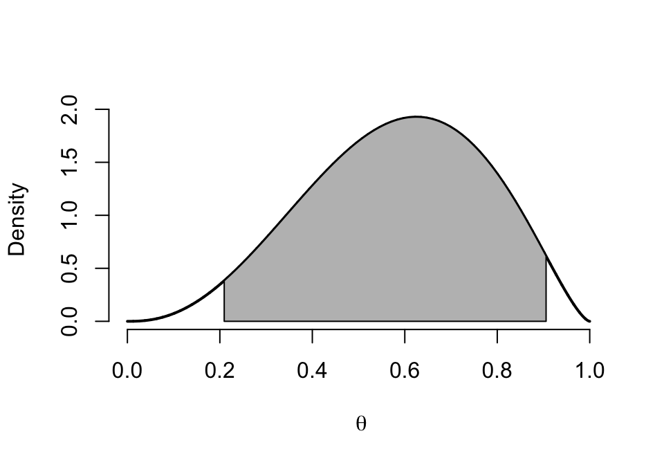
圖 42.8: Posterior distribution of Beta(3.5,2.5)
我們可以自己寫一個求可信區間的公式來計算:
# Credible Interval function:
# a, b : shape / super parameters
# level: probability level (0,1)

cred.int <- function(a,b,level){
  L <- qbeta((1-level)/2, a, b) # Lower limit
  U <- qbeta((1+level)/2, a, b) # Upper limit
  return(c(L,U))
}

cred.int(3.5,2.5,0.95)
## [1] 0.20941666 0.9056096795%可信區間 \((0.2094, 0.9056)\) 告訴我們,參數 \(\theta\in(0.2094, 0.9056)\) 的概率是 \(0.95\)。
下面我們嘗試寫 Beta 分佈的其他統計量:均值,衆數,方差等。
# a, b: shape / super parameters
MeanBeta <- function(a,b) a/(a+b)
ModeBeta <- function(a,b) {
  m <- ifelse(a>1 & b>1, (a-1)/(a+b-2), NA)
  return(m)
}
VarianceBeta <- function(a,b) (a*b)/((a+b)^2*(a+b+1))

# mean
MeanBeta(3.5,2.5)
## [1] 0.58333333## [1] 0.625## [1] 0.034722222## [1] 0.18633942.5.2 Q2
假如數據還是 Q1 的數據,然而先驗概率讓我們認爲可能在 5 名受試對象中觀察到 1 次事件。
- 試求超參數 \((a,b)\) 滿足先驗概率的 Beta 分佈。(不止一組)
解
我們認爲最有可能發生 “5 名受試對象中觀察到 1 次事件” 的情況,那麼先驗概率的均值爲 \(\frac{a}{a+b}=0.2\)。所以,在實數中有無數組超參數都可以用來模擬先驗概率分佈。例如 \(a=1, b=4; a=10, b=40; a=100, b=400; a=0.317, b=1.268, \cdots\)。
- 假如觀察數據是 \(n=5, r=1\),計算事後概率分佈及其均值,標準差。
解
先來嘗試寫一個計算貝葉斯二項分佈的方程:
# binbayes function in R
#------------------------------
# a, b: shape / super parameters
# r   : number of successes
# n   : number of trials

binbayes <- function(a, b, r, n) {
  prior <- c(a, b, NA, MeanBeta(a,b), sqrt(VarianceBeta(a, b)), qbeta(0.025, a, b), qbeta(0.5, a, b), qbeta(0.975, a, b))
  posterior <- c(a+r, b+n-r, r/n, MeanBeta(a+r, b+n-r), sqrt(VarianceBeta(a+r, b+n-r)), qbeta(0.025, a+r, b+n-r), qbeta(0.5, a+r, b+n-r), qbeta(0.975, a+r, b+n-r))
  out <- rbind(prior, posterior)
  out <- round(out, 4)
  colnames(out) <- c("a","b","r/n","Mean", "SD", "2.5%", "50%", "97.5%")
  return(out)
}

# a=1, b=4, r=1, n=5
binbayes(1,4,1,5)
## a b r/n Mean SD 2.5% 50% 97.5%
## prior 1 4 NA 0.2 0.1633 0.0063 0.1591 0.6024
## posterior 2 8 0.2 0.2 0.1206 0.0281 0.1796 0.4825## a b r/n Mean SD 2.5% 50% 97.5%
## prior 10 40 NA 0.2 0.0560 0.1024 0.1960 0.3202
## posterior 11 44 0.2 0.2 0.0535 0.1063 0.1963 0.3143通過繪製先驗概率分佈圖和事後概率分佈圖來比較二者的變化:
# Prior vs posterior graphs
# a,b : shape / super parameters
# r : number of successes
# n : number of trials
graph.binbayes <- function(a,b,r,n) {
prior <- Vectorize(function(theta) dbeta(theta, a,b))
posterior <- Vectorize(function(theta) dbeta(theta, a+r, b+n-r))
YL <- max(prior(seq(0.001,0.999,by=0.001)),posterior(seq(0.001,0.999,by=0.001)))
curve(prior, xlab=~theta, ylab="Density", lwd=1, lty=2,n=10000,ylim=c(0,YL), frame.plot = FALSE)
curve(posterior, xlab=~theta,lwd=2,lty = 1, add=T,n=10000)
}
graph.binbayes(1,4,1,5)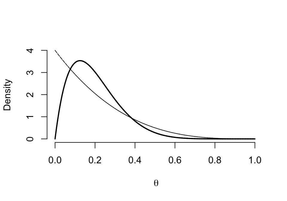
圖 42.9: Prior (dashed) Beta(1,4) vs. Posterior (cont.) Beta(2,8)
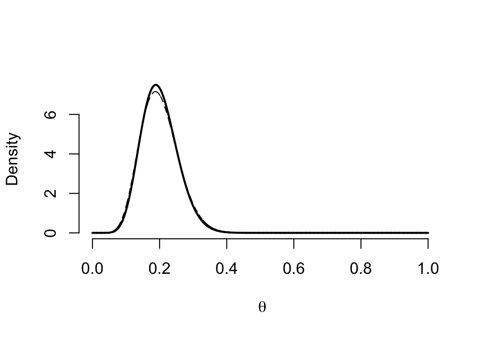
圖 42.10: Prior (dashed) Beta(10,40) vs. Posterior (cont.) Beta(11, 44)
我們可以很清楚的看見,先驗概率相同時,\(\text{Beta} (a,b)\) 的超參數如果越大,先驗概率的分佈就越趨近與對稱圖形,且極大值也就越出現在均值的地方 (本例中是 \(0.2\))。而且也會使事後概率的 HPD (highest posterior density) 的區間更狹窄 (意爲對事後概率的預測越準確),同時事後概率分佈也更加接近左右對稱。
42.5.3 Q3
我們事先估計某個事件在 \(n=20\) 名患者中發生的概率爲 \(15\%\)。當實際觀察數據爲 \(n=15,r=3\) 時,計算相應的事後概率。
解
# because 15% events happened in 20 subjects, assuming prior Beta(a=3, b=17)
# observed n=15, r=3
binbayes(3,17,3,15)## a b r/n Mean SD 2.5% 50% 97.5%
## prior 3 17 NA 0.1500 0.0779 0.0338 0.1383 0.3314
## posterior 6 29 0.2 0.1714 0.0628 0.0676 0.1651 0.3106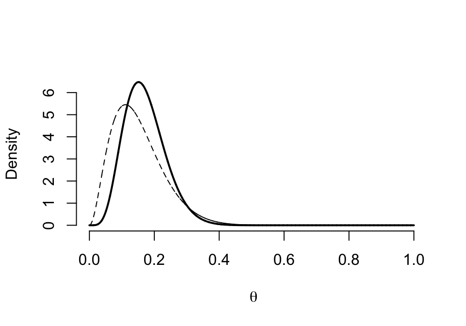
圖 42.11: Prior (dashed) Beta(3,17) vs. Posterior (cont.) Beta(6,29)
試着繪製先驗概率服從 \(\text{Beta} (1,1)\),回憶之前本章開頭的圖 42.7,這個先驗概率的含義就是我們沒有任何背景知識,對數據完全陌生的情況:
圖 42.12: Prior (dashed) Beta(1,1) vs. Posterior (cont.) Beta(4,13)
42.5.4 Q4
試給出上面各題中參數 \(\theta\) 落在 \((0.1,0.25)\) 之間的概率。
# function to calculate probabilities in a interval
# a, b: super parameters
# r : number of successes
# n : number of trials
# L : Lower limit of the probability interval
# U : Upper limit of the probability interval
prob.int <- function(a,b,r,n,L,U){
prior0 <- pbeta(U,a,b) - pbeta(L,a,b)
posterior0 <- pbeta(U,a+r,n-r+b) - pbeta(L,a+r,n-r+b)
prob <- as.matrix(c(prior0, posterior0))
prob <- round(prob,4)
colnames(prob) <- paste("Probability of theta lies between the Interval", L, U)
rownames(prob) <- c("Prior","Posterior")
return(prob)
}
# Prior Beta(0.317,1.286) n = 5, r=1
binbayes(0.317, 1.286, 1, 5)## a b r/n Mean SD 2.5% 50% 97.5%
## prior 0.317 1.286 NA 0.1978 0.2469 0.000 0.0823 0.8516
## posterior 1.317 5.286 0.2 0.1995 0.1449 0.013 0.1684 0.5493## Probability of theta lies between the Interval 0.1 0.25
## Prior 0.1711
## Posterior 0.3911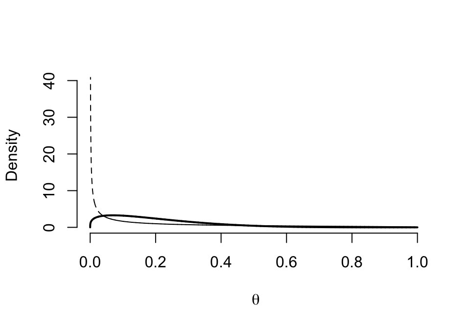
圖 42.13: Prior (dashed) Beta(0.317,1.286) vs. Posterior (cont.) Beta(1.317, 5.286)
##            a  b r/n Mean     SD   2.5%    50%  97.5%
## prior     10 40  NA  0.2 0.0560 0.1024 0.1960 0.3202
## posterior 11 44 0.2 0.2 0.0535 0.1063 0.1963 0.3143## Probability of theta lies between the Interval 0.1 0.25
## Prior 0.7951
## Posterior 0.8099所以在範圍固定的時候,事後概率分佈總是能夠比先驗概率分佈給出更高的累計概率。
42.5.5 Q5
一個臨牀試驗要進行兩個階段 (two phases),第一階段我們觀察到 \(10\) 個患者中 \(1\) 個事件。第二階段,觀察到 \(n=50, r=5\)。
- 兩個階段都使用 \(\text{Beta}(1,1)\) 作先驗概率。求兩個實驗階段參數 \(\theta<0.1\) 的概率。
##           a  b r/n   Mean     SD   2.5%   50%  97.5%
## prior     1  1  NA 0.5000 0.2887 0.0250 0.500 0.9750
## posterior 2 10 0.1 0.1667 0.1034 0.0228 0.148 0.4128## Probability of theta lies between the Interval 0 0.1
## Prior 0.1000
## Posterior 0.3026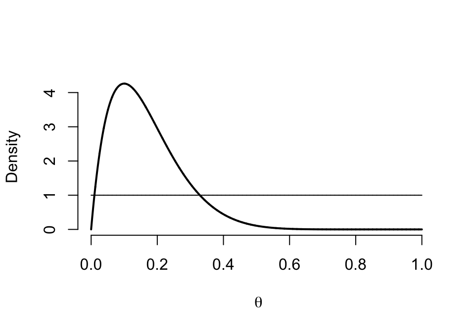
圖 42.14: Prior (dashed) Beta(1,1) vs. Posterior (cont.) Beta(2, 10)
##           a  b r/n   Mean     SD   2.5%    50%  97.5%
## prior     1  1  NA 0.5000 0.2887 0.0250 0.5000 0.9750
## posterior 6 46 0.1 0.1154 0.0439 0.0444 0.1105 0.2141## Probability of theta lies between the Interval 0 0.1
## Prior 0.1000
## Posterior 0.4024
圖 42.15: Prior (dashed) Beta(1,1) vs. Posterior (cont.) Beta(6, 46)
- 繼續使用先驗概率分佈 \(\text{Beta}(1,1)\),合併兩個實驗階段,求此時的事後概率分佈,以及參數 \(\theta<0.1\) 的概率。
##           a  b r/n   Mean     SD   2.5%    50%  97.5%
## prior     1  1  NA 0.5000 0.2887 0.0250 0.5000 0.9750
## posterior 7 55 0.1 0.1129 0.0399 0.0474 0.1087 0.2019## Probability of theta lies between the Interval 0 0.1
## Prior 0.1000
## Posterior 0.4105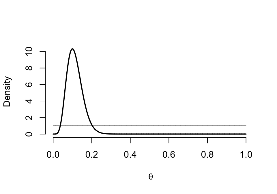
圖 42.16: Prior (dashed) Beta(1,1) vs. Posterior (cont.) Beta(7, 55)
- 用第一階段的實驗結果做第二階段實驗的先驗概率分佈,再計算事後概率分佈,以及 \(\theta<0.1\) 的概率。
##           a  b r/n   Mean     SD   2.5%    50%  97.5%
## prior     2 10  NA 0.1667 0.1034 0.0228 0.1480 0.4128
## posterior 7 55 0.1 0.1129 0.0399 0.0474 0.1087 0.2019## Probability of theta lies between the Interval 0 0.1
## Prior 0.3026
## Posterior 0.4105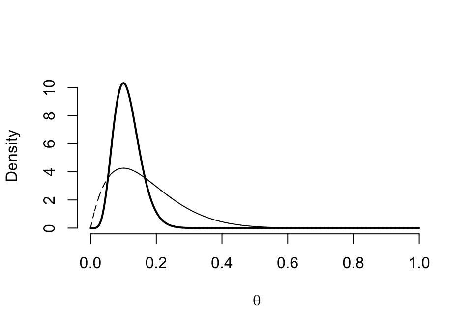
圖 42.17: Prior (dashed) Beta(2,10) vs. Posterior (cont.) Beta(7, 55)
第2,3兩個小問題提示我們,無論是將第一階段實驗結果作爲第二階段實驗的先驗假設還是將兩次實驗合併,最終的結果是不會改變的。Both approaches are equivalent.
42.5.6 Q6
藥物 A 和藥物 B 都被批准用於治療某種疾病。在 5000 例病例中使用藥物 A,發現有 3 人發生了不良副作用。在另外 7000 例病例中使用藥物 B,發現只有 1 例發生了副作用。
- 先使用單一分佈作爲先驗概率 (uniform prior: \(\text{Beta}(1,1)\))。求藥物 A 和藥物 B 各自發生不良反應的事後概率。
藥物 A
##           a    b    r/n   Mean     SD   2.5%    50%  97.5%
## prior     1    1     NA 0.5000 0.2887 0.0250 0.5000 0.9750
## posterior 4 4998 0.0006 0.0008 0.0004 0.0002 0.0007 0.0018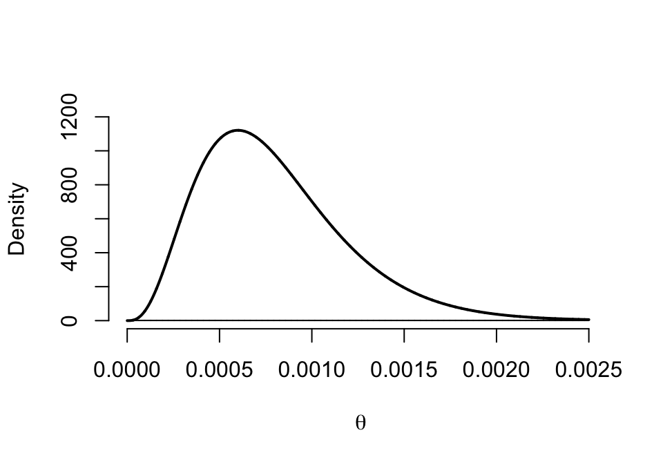
圖 42.18: Prior (dashed) Beta(1,1) vs. Posterior (cont.) Beta(4, 4998)
藥物 B
##           a    b    r/n   Mean     SD  2.5%    50%  97.5%
## prior     1    1     NA 0.5000 0.2887 0.025 0.5000 0.9750
## posterior 2 7000 0.0001 0.0003 0.0002 0.000 0.0002 0.0008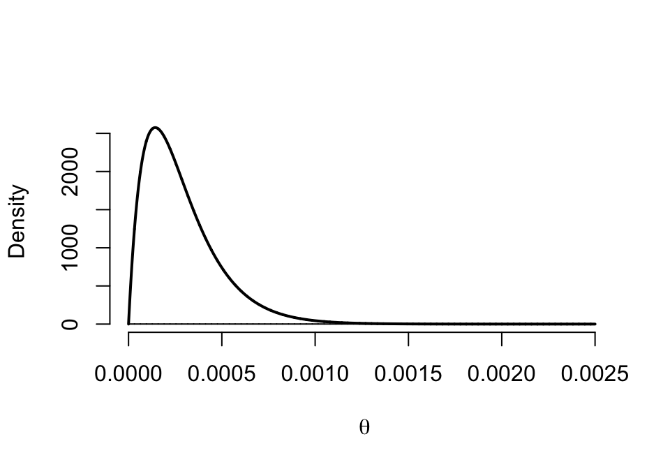
圖 42.19: Prior (dashed) Beta(1,1) vs. Posterior (cont.) Beta(2, 7000)
- 使用 \(\text{Beta}(0.00001,0.00001)\) 作爲先驗概率,重複上面的計算
藥物 A
##           a    b    r/n   Mean     SD   2.5%    50%  97.5%
## prior     0    0     NA 0.5000 0.5000 0.0000 0.5000 1.0000
## posterior 3 4997 0.0006 0.0006 0.0003 0.0001 0.0005 0.0014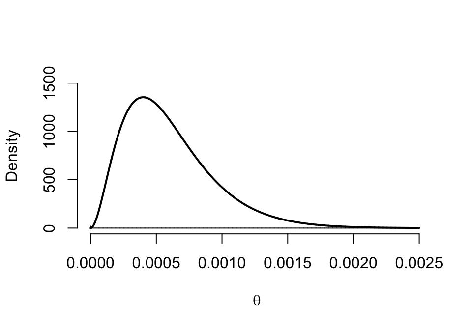
圖 42.20: Prior (dashed) Beta(0.00001,0.00001) vs. Posterior (cont.) Beta(3, 4997)
藥物 B
##           a    b    r/n   Mean     SD 2.5%    50%  97.5%
## prior     0    0     NA 0.5000 0.5000    0 0.5000 1.0000
## posterior 1 6999 0.0001 0.0001 0.0001    0 0.0001 0.0005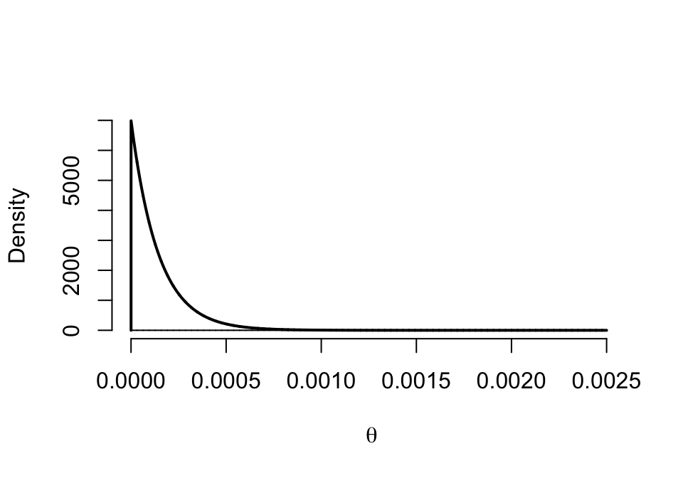
圖 42.21: Prior (dashed) Beta(0.00001,0.00001) vs. Posterior (cont.) Beta(1, 6999)
- 現在使用概率論的計算信賴區間 (confidence intervals) 的方法,求上面數據的精確二項分佈 95% 信賴區間。之前兩問中使用的哪個先驗概率更加接近概率論算法?
#------------------------------------------------
# Binomial confidence intervals
#------------------------------------------------
# r    : number of successes
# n    : number of trials
# level: confidence level
binom.confint <- function(r,n,level){
 p <- r/n
conf <-  as.vector(binom.test(r,n,conf.level = 0.95)$conf.int)
out <- c(p,conf)
out <- as.matrix(t(round(out,8)))
colnames(out) <- c("MLE", "L", "U")
return(out)
}

# Drug A
binom.confint(3,5000,0.95)
## MLE L U
## [1,] 0.0006 0.00012375 0.00175244## MLE L U
## [1,] 0.00014286 3.62e-06 0.00079569明顯可以看到,先驗概率使用 \(\text{Beta}(0.00001,0.00001)\) 時,事後概率的均值和可信區間的下限值更接近概率論算法。使用先驗概率 \(\text{Beta}(1,1)\) 時,事後概率的可信區間的上限值更接近概率論算法。
- 如果需要你來下結論說,藥物 B 和藥物 A 哪個更加安全? 求 \(\text{Pr}(\theta_B < \theta_A|data)\)。
解
貝葉斯
在計算機的輔助下,這是一個十分簡單的計算。我們從各自的事後分佈中採集大量隨機樣本,然後求 \(\theta_B-\theta_A\) 然後看有多少比例這個數值是小於零的就可以得出結論:
# Simulating from each posterior
set.seed(1001)
post.thetaA <- rbeta(1000000, 3, 4997)
post.thetaB <- rbeta(1000000, 1, 6999)

# Taking the differences
theta.diff0 <- post.thetaB - post.thetaA
# Histogram of the differences
hist(theta.diff0,probability = TRUE, breaks = 50, xlab=expression(theta[B] - theta[A]),main = "")
abline(v=0, col="red", lwd=2)
box()
圖 42.22: Histogram of Drug B - Drug A
也可以不採用直方圖而是使用連續曲線:
# Continuous version
plot(density(theta.diff0), xlab=expression(theta[B] - theta[A]), lwd=2, main = "", frame=FALSE)
abline(v=0, col="red", lwd=2)
box()
圖 42.23: Density of Drug B - Drug A
計算 \(\text{Pr}(\theta_B < \theta_A|data)\) 和可信區間:
## [1] 0.927829## 5% 95%
## -0.001142862872 0.000052484912## 10% 90%
## -0.00094605885 -0.00004674857# Simulating from each posterior
set.seed(1001)
post.thetaA <- rbeta(1000000, 4, 4998)
post.thetaB <- rbeta(1000000, 2, 7000)
# Taking the differences
theta.diff1 <- post.thetaB - post.thetaAhist(theta.diff1,probability = TRUE, breaks = 50, xlab=expression(theta[B] - theta[A]),main = "")
abline(v=0, col="red", lwd=2)
box()
圖 42.24: Histogram of Drug B - Drug A
# Continuous version
plot(density(theta.diff1), xlab=expression(theta[B] - theta[A]), lwd=2,main = "")
abline(v=0, col="red", lwd=2)
box()
圖 42.25: Density of Drug B - Drug A
計算 \(\text{Pr}(\theta_B < \theta_A|data)\) 和可信區間:
## [1] 0.899677## 5% 95%
## -0.00131289334 0.00013423126## 10% 90%
## -1.0955252e-03 6.5146438e-07概率論算法
# Normal Approximation
diff_mle <- (1/7000)-(3/5000)
diff_se <- sqrt( 1*6999/7000^3 + 3*4997/5000^3 )
U <- diff_mle + 1.28*diff_se
L <- diff_mle - 1.28*diff_se
print(c(U,L))
## [1] 0.000022358961 -0.000936644675# Comparison
plot(density(theta.diff0), xlab=expression(theta[B] - theta[A]), xlim= c(-0.002,0.001), lwd=2, col="red",main = "")
points(density(theta.diff1), xlab=expression(theta[B] - theta[A]), type = "l", col = "blue", lwd=2)
curve(norm.app,-0.0045,0.002,add=T,lwd=2,n=10000)
legend(-0.0021, 1300, c("Posterior with B(0,0)","Posterior with B(1,1)","Frequentist Normal App"), col=c("red","blue","black"),
text.col = "black", lty = c(1, 1, 1), lwd = c(2,2,2),
merge = TRUE, bg = "gray90",cex=0.8)
box()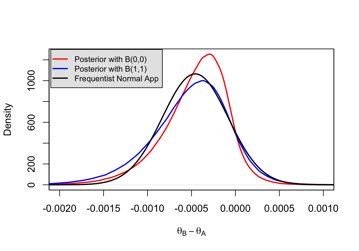
圖 42.26: Comparison of different prior distribution and frequentist approximation