第 45 章 多參數模型 Introduction to multiparameter models
45.1 把不需要的噪音參數平均出去 Averaging over ‘nuisance parameters’
從數學上表達聯合事後分佈 (joint posterior distribution) 和邊際事後分佈 (marginal posterior distribution) 其實不困難,可以想像我們想要了解的參數 \(\theta\) 其實是有兩個部分的,用 \(\theta = (\theta_1, \theta_2)\) 表示。更進一步想像,我們其實真正只對這兩部分參數中的其中一個 \(\theta_1\) 感興趣。那麼另一個就是所謂的“噪音參數 nuisance parameter”。例如我們在使用正(常)態分佈數據時,有兩個未知的參數,均值 \(\mu\),和方差 \(\sigma^2\)。但是實際上有時候我們可能只對其中一個感興趣,更多時候僅僅是均值,也有的時候是方差。
\[ y | \mu, \sigma^2 \sim N(\mu, \sigma^2) \]
那麼我們就需要尋找,其中一部分的參數在收集到的數據的條件下的分佈,\(p(\theta_1 | y)\)。
這裡需要仔細解釋一下如何求上述的數據條件參數分佈。當給定了數據 \(y\),通過微分思想,可以認為,未知參數 \(\theta\) 的期望值(或均值),可以通過在 \(y\) 的每一個小段的區間上的值的均值來獲得:
\[ E_{p(\theta | y)}[\theta] \approx \frac{1}{S}\sum_{S = 1}^S \theta^{(S)} \]
當這個區間 \(S \rightarrow 0\),也就是趨近於零時,上面的式子就轉化成了一個積分方程式:
\[ E_{p(\theta | y)}[\theta] \approx \frac{1}{S}\sum_{S = 1}^S \theta^{(S)} = \int\theta p(\theta | y) \]
那麼當參數不只一個的時候,它們的事後聯合分佈 (Joint posterior distribution),可以認為是:
\[ p(\theta_1, \theta_2 | y) \propto p(y | \theta_1, \theta_2) p(\theta_1, \theta_2) \]
之後的任務是要把 \(p(\theta_1, \theta_2 | y)\) 中的噪音參數 \(\theta_2\) 通過積分的方法去除掉。類似地,使用微分思想,我們把 \(p(\theta_2|y)\) 這個分佈分割成無數小的區間來計算每個區間裡的 \(\theta_1\),再求它的均值:
\[ p(\theta_1 |y) \approx \frac{1}{S} \sum_{S = 1}^S p(\theta_1, \theta_2^{(S)} | y) \] 其中,\(\theta_2\) 可以使用蒙特卡洛 (Monte Carlo) 過程從 \(p(\theta_2 | y)\) 中隨機採集。當這個無數小的區間的面積無限趨近於零時,\(S \rightarrow 0\),上面的方程式就變成了一個關於 \(\theta_2\) 的積分方程式:
\[ p(\theta_1 |y) \approx \frac{1}{S} \sum_{S = 1}^S p(\theta_1, \theta_2^{(S)} | y) = \int p(\theta_1, \theta_2 | y) d\theta_2 \]
這個過程被叫做邊際化 (marginalization)。進一步地,上面的積分方程中間的 \(p(\theta_1, \theta_2 | y)\) 又可以被理解成由兩個部分組成:一個是 \(p(\theta_1 | \theta_2, y)\),即增加了噪音參數 \(\theta_2\) 的條件事後分佈 (conditional posterior distribution given the nuisance parameter);另一個是 \(p(\theta_2 | y)\),也就是給定了數據 \(y\) 之後不同的 \(\theta_2\) 的取值的權重 (weighting function for the different possible values of \(\theta_2\)):
\[ p(\theta_1 | y) = \int p(\theta_1 |\theta_2 , y) p(\theta_2 | y) d\theta_2 \]
45.2 未知均值也未知方差的正(常)態分佈數據 normal data with unknown mean and variance
作為一個經典的例子,我們思考從數據中估計一個未知的平均值。假設該數據是一維的 \(n\) 個獨立樣本 \(y\) 服從正(常)態分佈 \(N(\mu, \sigma^2)\)。
45.2.1 無信息先驗概率分佈 noninformative prior distribution
根據 Jeffreys prior 對無信息先驗概率分佈的定義,我們給這個未知均值也未知方差的數據的兩個參數的無信息先驗概率分佈分別是:均值 \(\mu\) 使用均一分佈 (uniform distribution),方差 \(\sigma^2\) 使用 \(\sigma^{-2}\):
\[ p(\mu, \sigma^2) \propto \sigma^{-2} \]
於是,該數據的聯合事後概率分佈可以被推導為:
\[ \begin{aligned} p(\mu, \sigma^2 | y) & \propto \sigma^{-2} \prod_{i =1}^n \frac{1}{\sqrt{2\pi} \sigma} \exp\left( -\frac{1}{2\sigma^2}(y_i - \mu)^2 \right) \\ & = \sigma^{-n - 2} \exp\left(-\frac{1}{2\sigma^2}\sum_{i =1}^n (y_i - \mu)^2 \right) \\ & = \sigma^{-n - 2} \exp\left(-\frac{1}{2\sigma^2}\sum_{i =1}^n (y_i^2 - 2y_i\mu + \mu^2) \right) \\ & = \sigma^{-n - 2} \exp\left(-\frac{1}{2\sigma^2}\sum_{i =1}^n (y_i^2 - 2y_i\mu + \mu^2 -\bar{y}^2 + \bar{y}^2 - 2y_i\bar{y} + 2y_i\bar{y} ) \right) \\ & = \sigma^{-n - 2} \exp\left(-\frac{1}{2\sigma^2}\left[\sum_{i =1}^n (y_i^2 - 2y_i\bar{y} + \bar{y}^2) + \sum_{i = 1}^n(\mu^2 - 2y_i\mu - \bar{y}^2 + 2y_i\bar{y}) \right]\right) \\ & = \sigma^{-n - 2} \exp\left(-\frac{1}{2\sigma^2}\left[\sum_{i =1}^n (y_i^2 - 2y_i\bar{y} + \bar{y}^2) + n(\mu^2 - 2\bar{y}\mu - \bar{y}^2 + 2\bar{y}^2) \right]\right) \\ & = \sigma^{-n - 2} \exp\left(-\frac{1}{2\sigma^2}\left[\sum_{i =1}^n (y - \bar{y})^2 + n(\bar{y} - \mu)^2 \right]\right) \\ \color{darkred}{\text{Where } \bar{y}} & \color{darkred}{= \frac{1}{n}\sum_{i = 1}^n y_i} \\ & = \sigma^{-n - 2} \exp\left(-\frac{1}{2\sigma^2}\left[(n - 1)s^2 + n(\bar{y} - \mu)^2 \right]\right) \\ \color{darkred}{\text{Where } s^2} & \color{darkred}{= \frac{1}{n - 1}\sum_{i = 1}^n (y_i - \bar{y})^2} \\ \end{aligned} \]
此時,其實我們有兩種邊際分佈選擇,一種是把方差作為噪音參數,另一種是把均值作為噪音參數。先是 \(\mu\) 的邊際分佈,它是通過把 \(\sigma\) 積分出去獲得的:
\[ p(\mu | y) = \int p(\mu, \sigma^2 | y) d\sigma^2 \]
其次是 \(\sigma^2\) 的邊際分佈,它是通過把 \(\mu\) 積分出去獲得的:
\[ p(\sigma^2 | \mu) = \int p(\mu, \sigma^2 | y) d \mu \]
下面我們來推導把均值積分出去的過程:
\[ \begin{aligned} p(\sigma^2 | y) & \propto \int p(\mu, \sigma^2 | y) d \mu \\ & \propto \int \sigma^{-n - 2} \exp\left(-\frac{1}{2\sigma^2}\left[(n - 1)s^2 + n(\bar{y} - \mu)^2 \right]\right) d\mu \\ \text{Move terms } & \text{does not include } \mu \text{ outside of the intergral } \\ & \propto \sigma^{-n - 2} \exp\left( -\frac{1}{2\sigma^2}(n - 1)s^2 \right) \int\exp\left( -\frac{n}{2\sigma^2}(\bar{y} - \mu)^2 \right) d\mu \\ \because \int \frac{1}{\sqrt{2\pi\sigma^2}} & \exp\left(- \frac{1}{2\sigma^2}(y - \theta) \right)d\theta = 1 \text{ integration of the pdf of a normal distribution} \\ & \propto \sigma^{-n - 2} \exp\left( -\frac{1}{2\sigma^2}(n - 1)s^2 \right) \times \sqrt{\frac{2\pi\sigma^2}{n}} \\ & \propto (\sigma^2)^{-(\frac{n -1}{2} + 1)} \exp\left( -\frac{(n -1 )s^2}{2\sigma^2} \right) \end{aligned} \] 你會發現這個邊際分佈的概率函數竟然成了一個逆卡方分佈:
\[ p(\sigma^2 | y) = \text{Inv-}\chi^2 (\sigma^2 | n - 1, s^2) \]
對比正常態分佈數據已知均值,求它方差的邊際分佈的時候我們用到的逆卡方分佈的特徵值如下 (參考 Chapter 44.1):
\[ \begin{aligned} \sigma^2 | y & \sim \text{Inv-}\chi^2(\sigma^2| n, v) \\ \text{Where } v & = \frac{1}{n}\sum_{i =1}^n(y_i - \theta)^2 \end{aligned} \]
而此時我們推導出的未知均值,需要用樣本均值來估計時的方差邊際分佈為:
\[ \begin{aligned} \sigma^2 | y & \sim \text{Int-}\chi^2(n - 1, s^2) \\ \text{Where } s^2 & = \frac{1}{n -1}\sum_{i = 1}^n(y_i - \bar{y})^2 \end{aligned} \]
也就是說,在均值未知時,由於此時需要對均值作額外的估計,它本身的不確定性使得方差在估計的時候也增加了不確定性(雙側尾部變厚)。
所以,一個未知均值也未知方差的正常態分佈數據,我們採集兩個未知參數的事後概率分佈的過程其實可以描述成為下面的過程:
\[ \begin{aligned} \text{The posterior} & \text{ joint distribution is:} \\ p(\mu, \sigma^2 | y) & = \color{darkred}{p(\mu | \sigma^2, y)} \color{darkgreen}{p(\sigma^2 | y)} \\ \color{darkgreen}{p(\sigma^2 | y)} & = \text{Inv-}\chi^2 (\sigma^2 | n-1, s^2) \\ (\sigma^2)^{(s)} & \sim \color{darkgreen}{p(\sigma^2 | y)} \\ \color{darkred}{p(\mu | \sigma^2, y)} & = N(\mu | \bar{y}, \sigma^2 /n) \color{grey}{\propto \exp\left( -\frac{n}{2\sigma^2}(\bar{y} - \mu)^2 \right)} \\ \mu^{(s)} & \sim \color{darkred}{p(\mu | \sigma^2, y)} \\ \mu^{(s)}, (\sigma^2)^{(s)} & \sim p(\mu, \sigma^2 | y) \end{aligned} \]
45.2.2 均值的事後邊際概率分佈 marginal posterior distribution of \(\mu\)
通常我們在均值和方長二者之間會更關心總體的均值 (population mean) \(\mu\)。那麼通過把方差從二者的事後聯合分佈中積分出去的方法,可以獲得:
\[ \begin{aligned} p(\mu | y) & = \int_0^\infty p(\mu, \sigma^2 |y) d\sigma^2 \\ & \propto \int_0^\infty \sigma^{-n - 2} \exp\left(-\frac{1}{2\sigma^2}\left[(n - 1)s^2 + n(\bar{y} - \mu)^2 \right]\right) d\sigma^2 \end{aligned} \]
對上述函數進行簡化的過程中,需要用到下面的轉換輔助理解其過程:
\[ A = (n - 1)s^2 + n(\bar{y} - \mu)^2 \text{ and } z = \frac{A}{2\sigma^2} \]
那麼上面的公式可以被修改成關於 \(z\) 的積分函數:
\[ \begin{aligned} p(\mu | y) & \propto A^{-n/2} \int_0^\infty z^{(n - 2)/2} \exp(-z)dz \\ \color{gray}{\text{Recognize }}& \color{gray}{\text{Gamma intergral }\Gamma(u) = \int_0^\infty x^{u-1}\exp(-x)dx} \\ \color{gray}{\text{Although t}}& \color{gray}{\text{here are different power terms, }} \\ \color{gray}{\text{but we kno}}& \color{gray}{\text{w this intergral will give us a constant value.}} \\ \color{gray}{\text{therefore o}}& \color{gray}{\text{nly the } A \text{ part is left in the proporional portions}} \\ & \propto \left[ (n - 1)s^2 + n(\bar{y} - \mu)^2 \right]^{-n/2} \\ & \propto \left[ 1 + \frac{n(\bar{y} - \mu)^2}{(n - 1)s^2} \right]^{-n/2} \\ \Rightarrow p(\mu | y) & \propto t_{n-1}(\mu | \bar{y}, \frac{s^2}{n}) \color{gray}{\text{ is a Student's } t \text{ distribution}} \end{aligned} \] 我們成功推導出未知方差未知均值的正常態數據的事後概率分佈是一個 \(t\) 分佈。
45.3 R 演示 正常態數據但均值方差均未知
參考原著作者代碼
- 一串可能是正常態分佈的數據
- 該數據的充分統計量
- 我們希望採集樣本的事後聯合分佈可以被理解為兩個條件分佈的乘積:
\[ p(\mu, \sigma^2 | y) = p(\sigma^2 | y) p(\mu | \sigma^2, y) \]
由於我們知道方差的事後概率分佈是逆縮放卡方分佈 (scaled inverse chi-squared distribution),我們需要兩個輔助函數,一個是隨機採樣函數,一個是概率密度函數:
# random sampler for scaled inverse chi-squared distribution
rsinvchisq <- function(n, nu, s2, ...) nu*s2 / rchisq(n, nu, ...)

# probabilityb density function for scaled inverse chi-squared distribution
dsinvchisq <- function(x, nu, s2){
        exp(log(nu/2)*nu/2 - lgamma(nu/2) + log(s2)/2*nu - log(x)*(nu/2+1) - (nu*s2/2)/x)
}

# 上述概率密度函數其實是把縮放逆卡方分佈的概率密度函數本身先取對數,再作 exp 提高計算效率- 從 \(p(\sigma^s | y)\) 中採集 1000 個樣本
- 從 \(p(\mu | \sigma^2 , y)\) 中採集樣本
mu <- rnorm(ns, my, sqrt(sigma2/n))
# or equivalently
# mu <- my + sqrt(sigma2/n)*rnorm(length(sigma2)- 從預測分佈中採集樣本 \(p(\tilde{y} | y)\)
- 為計算
sigma, mu, ynew在一些範圍內的小區隔之間的密度準備
t1l <- c(90, 150)
t2l <- c(10, 60)
nl <- c(50, 185)
t1 <- seq(t1l[1], t1l[2], length.out = ns)
t2 <- seq(t2l[1], t2l[2], length.out = ns)
xynew <- seq(nl[1], nl[2], length.out = ns)- 計算 \(\mu\) 的精確邊際分佈密度 (the exact marginal density of \(p(\mu)\)),記得它是一個自由度為 \(n-1\) 的 t 分佈。
# multiplication by 1./sqrt(s2/n) is due to the transformation of
# variable z=(x-mean(y))/sqrt(s2/n)
pm <- dt((t1-my) / sqrt(s2/n), n-1) / sqrt(s2/n)- 從採集的均值樣本推算以這些均值的高斯內核近似估計:(estimate the marginal density using samples and ad hoc Gaussian kernel approximation)
- 類似地,計算標準差本身的精確邊際分佈密度 (the marginal density of \(p(\sigma^2)\)),它是一個逆縮放卡方分佈,自由度是 \(n-1\),縮放尺度是 \(s^2\)
# the multiplication by 2*t2 is due to the transformation of
# variable z=t2^2, see BDA3 p. 21
ps <- dsinvchisq(t2^2, n-1, s2) * 2*t2- 計算採集得到的事後標準差樣本本身的高斯內核估計 (estimate the marginal density using samples and ad hoc Gaussian kernel approximation)
- 計算精確的預測值本身的分佈密度 (compute the exact predictive density)
# multiplication by 1./sqrt(s2/n) is due to the transformation of variable
# see BDA3 p. 21
p_new <- dt((xynew-my) / sqrt(s2*(1+1/n)), n-1) / sqrt(s2*(1+1/n))- 估計事後聯合分佈的密度。
# Combine grid points into another data frame
# with all pairwise combinations
dfj <- data.frame(t1 = rep(t1, each = length(t2)),
                  t2 = rep(t2, length(t1)))
dfj$z <- dsinvchisq(dfj$t2^2, n-1, s2) * 2*dfj$t2 * dnorm(dfj$t1, my, dfj$t2/sqrt(n))
# breaks for plotting the contours
cl <- seq(1e-5, max(dfj$z), length.out = 6)
45.3.1 繪製聯合事後密度分佈及均值和方差各自的邊際分佈 visualise the joint and marginal densities
- 下面的代碼用於生成均值的邊際分佈
dfm <- data.frame(t1, Exact = pm, Empirical = pmk) %>% gather(grp, p, -t1)
margmu <- ggplot(dfm) +
  geom_line(aes(t1, p, color = grp)) +
  coord_cartesian(xlim = t1l) +
  labs(title = 'Marginal of mu', x = '', y = '') +
  scale_y_continuous(breaks = NULL) +
  theme(legend.background = element_blank(),
        legend.position = c(0.75, 0.8),
legend.title = element_blank())- 下面的代碼用於生成標準差的邊際分佈
dfs <- data.frame(t2, Exact = ps, Empirical = psk) %>% gather(grp, p, -t2)
margsig <- ggplot(dfs) +
  geom_line(aes(t2, p, color = grp)) +
  coord_cartesian(xlim = t2l) +
  coord_flip() +
  labs(title = 'Marginal of sigma', x = '', y = '') +
  scale_y_continuous(breaks = NULL) +
  theme(legend.background = element_blank(),
        legend.position = c(0.75, 0.8),
        legend.title = element_blank())
## Coordinate system already present. Adding new coordinate system, which will replace the existing one.- 下面的代碼用於繪製聯合事後分佈密度
joint1labs <- c('Samples','Exact contour')
joint1 <- ggplot() +
  geom_point(data = data.frame(mu,sigma), aes(mu, sigma, col = '1'), size = 0.1) +
  geom_contour(data = dfj, aes(t1, t2, z = z, col = '2'), breaks = cl) +
  coord_cartesian(xlim = t1l,ylim = t2l) +
  labs(title = 'Joint posterior', x = '', y = '') +
  scale_y_continuous(labels = NULL) +
  scale_x_continuous(labels = NULL) +
  scale_color_manual(values=c('blue', 'black'), labels = joint1labs) +
  guides(color = guide_legend(nrow  = 1, override.aes = list(
    shape = c(16, NA), linetype = c(0, 1), size = c(2, 1)))) +
  theme(legend.background = element_blank(),
        legend.position = c(0.5, 0.9),
legend.title = element_blank())- 合併上面三個圖

圖 45.1: The joint density and marginal densities of the posterior of normal distribution with unknown mean and variance
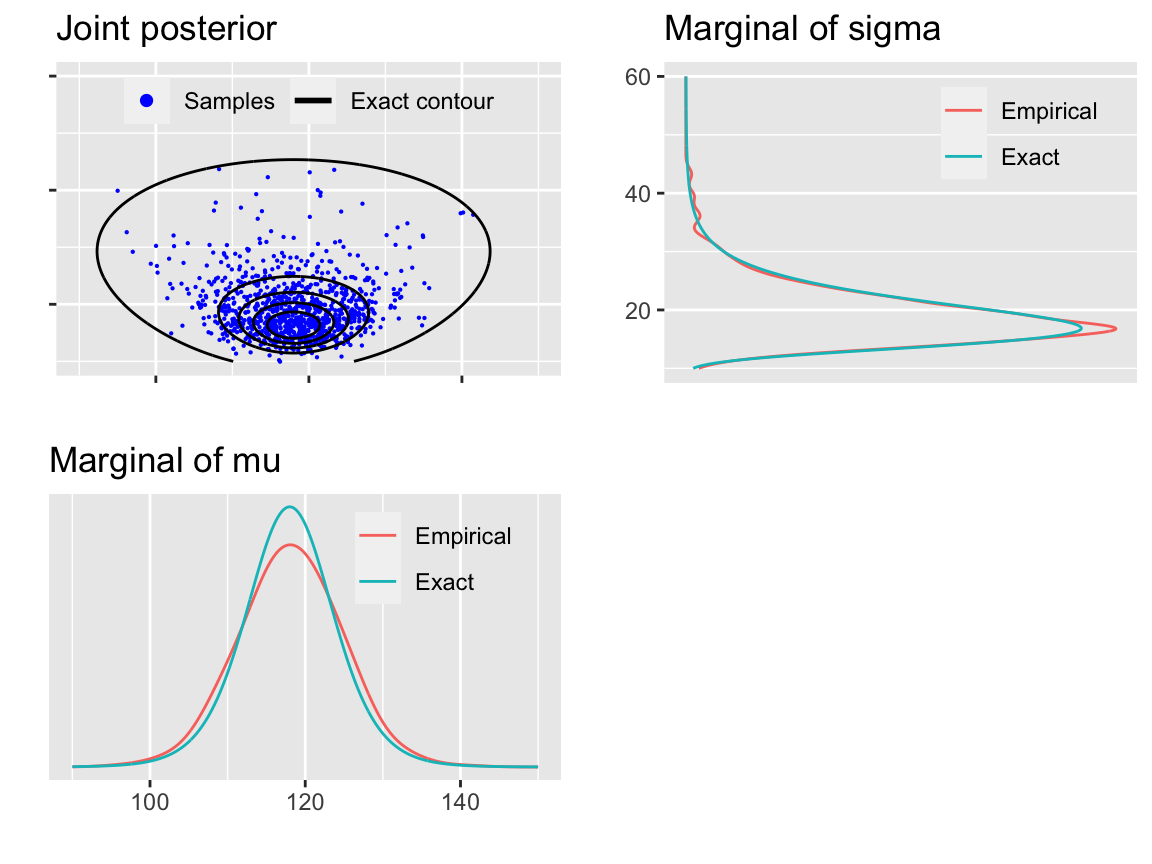
圖 45.2: The joint density and marginal densities of the posterior of normal distribution with unknown mean and variance
45.3.2 單獨繪製邊際分佈的每一個部分
- 繪製另外一個聯合事後分佈橢圓等高線圖
# data frame for the conditional of mu and marginal of sigma
dfc <- data.frame(mu = t1, marg = rep(sigma[1], length(t1)),
                  cond = sigma[1] + dnorm(t1 ,my, sqrt(sigma2[1]/n)) * 100) %>%
  gather(grp, p, marg, cond)
# legend labels for the following plot
joint2labs <- c('Exact contour plot', 'Sample from joint post.',
               'Cond. distribution of mu', 'Sample from the marg. of sigma')
joint2 <- ggplot() +
  geom_contour(data = dfj, aes(t1, t2, z = z, col = '1'), breaks = cl) +
  geom_point(data = data.frame(m = mu[1], s = sigma[1]), aes(m , s, color = '2')) +
  geom_line(data = dfc, aes(mu, p, color = grp), linetype = 'dashed') +
  coord_cartesian(xlim = t1l,ylim = t2l) +
  labs(title = 'Joint posterior', x = '', y = '') +
  scale_x_continuous(labels = NULL) +
  scale_color_manual(values=c('blue', 'darkgreen','darkgreen','black'), labels = joint2labs) +
  guides(color = guide_legend(nrow  = 2, override.aes = list(
    shape = c(NA, 16, NA, NA), linetype = c(1, 0, 1, 1)))) +
  theme(legend.background = element_blank(),
        legend.position = c(0.5, 0.85),
legend.title = element_blank())- 繪製標準差的邊際密度函數
margsig2 <- ggplot(data = data.frame(t2, ps)) +
  geom_line(aes(t2, ps), color = 'blue') +
  coord_cartesian(xlim = t2l) +
  coord_flip() +
  labs(title = 'Marginal of sigma', x = '', y = '') +
  scale_y_continuous(labels = NULL)
## Coordinate system already present. Adding new coordinate system, which will replace the existing one.- 合併兩個圖
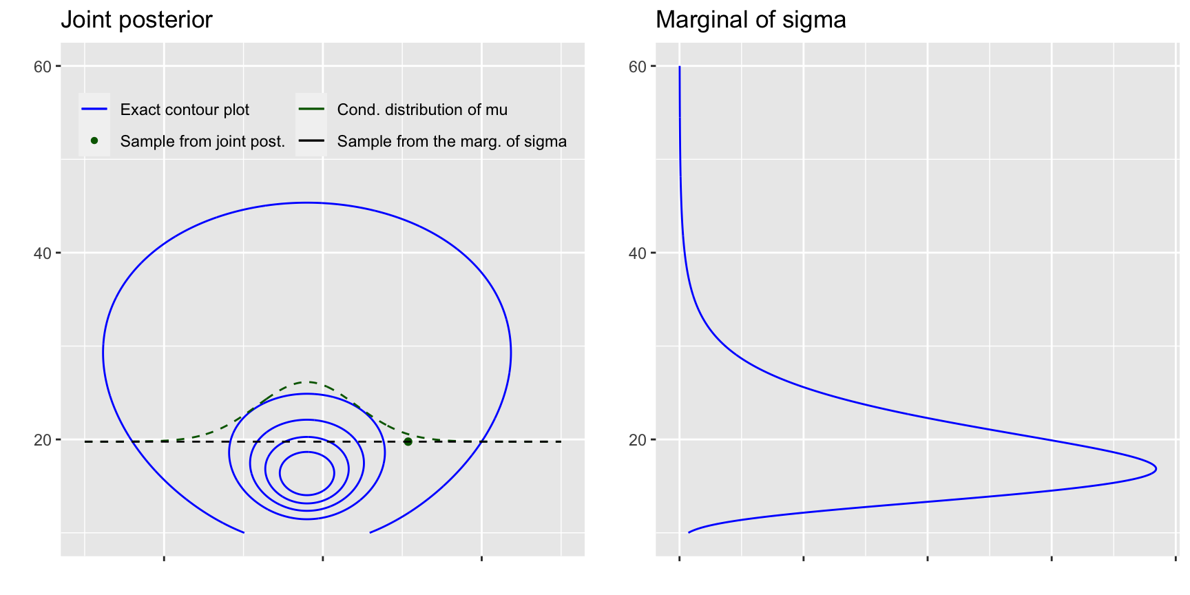
圖 45.3: Visualise factored sampling and the corresponding marginal and conditional densities.
45.3.3 繪製事後均值的概率密度分佈
- 計算每一個樣本的概率密度分佈
- 繪製其中25個樣本
# data frame of 25 first samples
dfm25 <- data.frame(t1, t(condpdfs[1:25,])) %>% gather(grp, p, -t1)
condmu <- ggplot(data = dfm25) +
  geom_line(aes(t1, p, group = grp), linetype = 'dashed') +
  labs(title = 'Conditional distribution of mu for first 25 samples', y = '', x = '') +
scale_y_continuous(breaks = NULL)- 繪製這些事後均值樣本的均值
dfsam <- data.frame(t1, colMeans(condpdfs), pm) %>% gather(grp,p,-t1)
# labels
mulabs <- c('avg of sampled conds', 'exact marginal of mu')
meanmu <- ggplot(data = dfsam) +
  geom_line(aes(t1, p, size = grp, color = grp)) +
  labs(y = '', x = 'mu') +
  scale_y_continuous(breaks = NULL) +
  scale_size_manual(values = c(2, 0.8), labels = mulabs) +
  scale_color_manual(values = c('orange', 'black'), labels = mulabs) +
  theme(legend.position = c(0.8, 0.8),
        legend.background = element_blank(),
legend.title = element_blank())- 合併
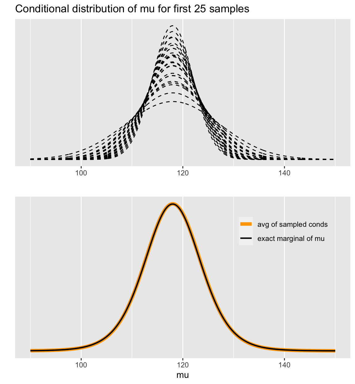
圖 45.4: Visualise the marginal distribution of mu
45.4 R 演示 分析二進制數據 (BDA3 P.74)
在藥物研發,或者化學物品毒性測量的試驗中,常常需要對試驗動物使用不同的藥物或者毒性劑量做劑量反應試驗。一般來說,動物試驗的時候我們多數情況下會使用死亡/生存,或者發生腫瘤/未發生腫瘤作為該劑量反應觀察的結果。這樣的實驗獲得的數據結果基本上是這樣形式的:
\[ (x_i, n_i, y_i); i = 1, \dots, k \] 其中,
- \(k\) 是藥物/毒物劑量水平的分組;
- \(x_i\) 是第 \(i\) 劑量組的實際藥物濃度,通常會取對數;
- \(n_i\) 是第 \(i\) 劑量組的實驗動物數量;
- \(y_i\) 是第 \(i\) 劑量組的實驗動物死亡(或發現腫瘤的動物)數量。
某個實驗的結果如下,實驗一共使用了20只動物,其中每個劑量組有五隻,每個劑量組死亡動物數分別是 0, 1, 3, 5:
##       x n y
## 1 -0.86 5 0
## 2 -0.30 5 1
## 3 -0.05 5 3
## 4  0.73 5 5
根據我們的假設,第 \(i\) 劑量組內的實驗動物本身是可以替換的 (exchangeable),相互獨立的 (independent),死亡概率應該在相同的劑量下是相同的 (equal probabilities),那麼這樣的數據測量到的 \(y_i\) 是一個典型的服從二項分佈的數據:
\[ y_i|\theta_i \sim \text{Bin}(n_i, \theta_i) \]
其中,
- \(\theta_i\) 是第\(i\)劑量組實驗動物的死亡概率,該組劑量是 \(x_i\);
那麼該數據的標準解決方案是使用羅輯回歸模型:
\[ \begin{equation} \text{logit}(\theta_i) = \log(\frac{\theta_i}{1 - \theta_i})\\ \text{logit}(\theta_i) = \alpha + \beta x_i \end{equation} \tag{45.1} \]
- 繪製該數據的散點圖
ggplot(df1, aes(x=x, y=y)) +
    geom_point(size=2, color='red') +
    scale_x_continuous(breaks = df1$x, minor_breaks=NULL, limits = c(-1.5, 1.5)) +
    scale_y_continuous(breaks = 0:5, minor_breaks=NULL) +
    labs(title = 'Bioassay', x = 'Dose (log g/ml)', y = 'Number of deaths') +
    theme(panel.grid.major = element_blank())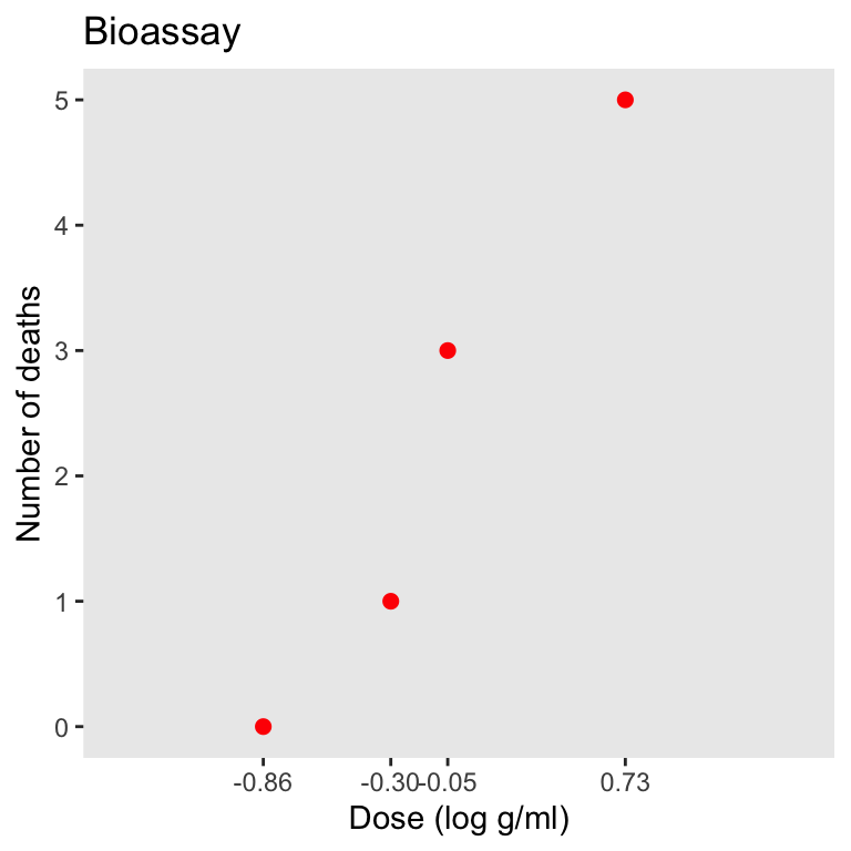
圖 45.5: The Bioassay example data.
根據該數據的模型函數 (Model (45.1)),我們可以寫下本數據的似然 likelihood:
\[ \begin{equation} p(y_i|\alpha, \beta) \propto \left[ \text{logit}^{-1}(\alpha + \beta x_i) \right]^{y_i}\left[ 1- \text{logit}^{-1}(\alpha + \beta x_i) \right]^{n_i - y_i} \end{equation} \tag{45.2} \]
於是該模型的事後概率分佈為:
\[ \begin{aligned} p(\alpha, \beta | y) & \propto p(\alpha, \beta) p(y | \alpha, \beta) \\ & \propto p(\alpha, \beta) \prod_{i = 1}^k p(y | \alpha, \beta) \end{aligned} \tag{45.3} \]
為了便於計算,可推導似然函數 (Likelihood function (45.2)) 變成如下的對數似然 (log-likelihood):
\[ \ell_i \propto y_i(\alpha + \beta x_i) - n_i \log\left[ 1 + \exp(\alpha + \beta x_i) \right] \] - 在 R 裡設定好這個對數似然函數:
- 設定參數 \(\alpha, \beta\) 可能的範圍,然後準備好用於事後概率密度採樣使用的小格子
A = seq(-4, 8, length.out = 50)
B = seq(-10, 40, length.out = 50)
cA <- rep(A, each = length(B))
cB <- rep(B, length(A))- 計算該數據
df1的似然:
- 從這些小格子裡根據似然來採集樣本(with replacement)
nsamp <- 1000
samp_indices <- sample(length(p), size = nsamp,
                       replace = T, prob = p/sum(p))
samp_A <- cA[samp_indices[1:nsamp]]
samp_B <- cB[samp_indices[1:nsamp]]

# Add random jitter, see BDA3 p. 76

samp_A <- samp_A + runif(nsamp, (A[1] - A[2])/2, (A[2] - A[1])/2)
samp_B <- samp_B + runif(nsamp, (B[1] - B[2])/2, (B[2] - B[1])/2)- 生成樣本數據
- 繪製採集的邏輯曲線
invlogit <- plogis
xr <- seq(-1.5, 1.5, length.out = 100)
dff <- pmap_df(samps[1:100,], ~ tibble(x = xr, id=..1,
                                   f = invlogit(..2 + ..3*x)))
ppost <- ggplot(df1, aes(x=x, y=y/n)) +
  geom_line(data=dff, aes(x=x, y=f, group=id), linetype=1, color='blue', alpha=0.2) +
  geom_point(size=2, color='red') +
  scale_x_continuous(breaks = df1$x, minor_breaks=NULL, limits = c(-1.5, 1.5)) +
  scale_y_continuous(breaks = seq(0,1,length.out=3), minor_breaks=NULL) +
  labs(title = 'Bioassay', x = 'Dose (log g/ml)', y = 'Proportion of deaths') +
  theme(panel.grid.major = element_blank())

# add 50% death line and LD50 dots
ppost + geom_hline(yintercept = 0.5, linetype = 'dashed', color = 'gray') +
  geom_point(data=samps[1:100,], aes(x=ld50, y=0.5), color='blue', alpha=0.2)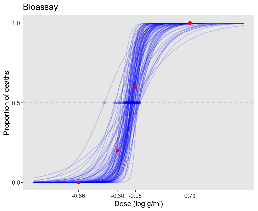
圖 45.6: Draws of logistic curves of the bioassay data, with 50% deaths line and LD50 dots.
- 繪製事後概率密度圖
# limits for the plots
xl <- c(-2, 8)
yl <- c(-2, 40)
pos <- ggplot(data = data.frame(cA ,cB, p), aes(cA, cB)) +
  geom_raster(aes(fill = p, alpha = p), interpolate = T) +
  geom_contour(aes(z = p), colour = 'black', size = 0.2) +
  coord_cartesian(xlim = xl, ylim = yl) +
  labs(title = 'Posterior density evaluated in grid', x = 'alpha', y = 'beta') +
  scale_fill_gradient(low = 'yellow', high = 'red', guide = F) +
  scale_alpha(range = c(0, 1), guide = F)

sam <- ggplot(data = samps) +
  geom_point(aes(alpha, beta), color = 'blue') +
  coord_cartesian(xlim = xl, ylim = yl) +
  labs(title = 'Posterior draws', x = 'alpha', y = 'beta')
grid.arrange(pos, sam, nrow=2)
## Warning: It is deprecated to specify `guide = FALSE` to remove a guide. Please use `guide = "none"` instead.
## It is deprecated to specify `guide = FALSE` to remove a guide. Please use `guide = "none"` instead.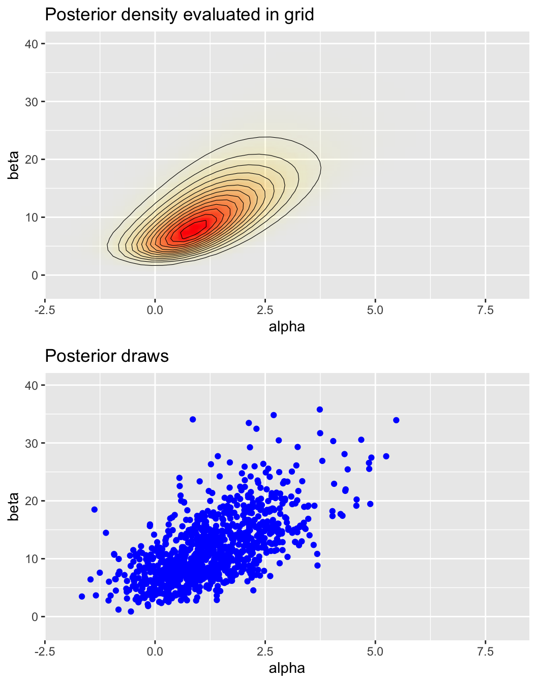
圖 45.7: Plot of the posterior joint density.
- 繪製事後 LD50 的直方圖,這裡 LD50 的含義是,在多大的濃度時,動物死亡/發生腫瘤的概率會是50%。
his <- ggplot(data = samps) +
  geom_histogram(aes(ld50), binwidth = 0.02,
                 fill = 'steelblue', color = 'black') +
  coord_cartesian(xlim = c(-0.5, 0.5)) +
  labs(x = 'LD50 = -alpha/beta')
his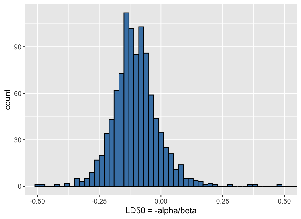
圖 45.8: Histogram of the draws from the posterior distribution of LD50 on the scale of log dose in g/ml.