第 117 章 從流行病學的角度初步分析生存數據 introduction to survival analysis
在本次練習題中,我們學習如何繪製 Kaplan-Meier 生存曲線,並且學會使用 Logrank 檢驗方法來比較不同組之間的生存曲線是否有統計學上的不一致。
117.1 Q1
打開數據 trinmlsh。使用 Stata 的 describe 和 sum 命令熟悉該數據的各個變量的名字和大致內容。主要是確認一下哪些變量含有重要的結果變量信息,和生存時間信息。help trinmlsh 可以調取關於該數據更加詳細的背景和內容介紹。
##
## . cd "~/Downloads/LSHTMlearningnote/backupfile/Users/chaoimacmini/Downloads/LSHTMlearningnote/backupfiles
##
## . use trinmlsh
##
## .
## . describe
##
## Contains data from trinmlsh.dta
##   obs:           318
##  vars:            18                          14 Sep 1999 11:20
## -------------------------------------------------------------------------------
##               storage   display    value
## variable name   type    format     label      variable label
## -------------------------------------------------------------------------------
## ethgp           float   %9.0g      lethgp     Ethnic group
## ageent          float   %9.0g                 Age in years at first survey
## death           float   %9.0g                 Died from any cause
## cvdeath         float   %9.0g                  Died from CV disease
## alc             float   %9.0g      lalc       drinks per week
## smokenum        float   %9.0g      lsmokn     No. of cigarettes per day
## hdlc            float   %9.0g                 HDL cholesterol
## diabp           float   %9.0g                 Diastolic blood pressure
## sysbp           float   %9.0g                 Systolic blood pressure
## chdstart        float   %9.0g                 Heart disease at time of entry
## days            float   %9.0g
## years           float   %9.0g
## bmi             float   %9.0g
## id              float   %9.0g
## timein          float   %d
## timeout         float   %d
## y               float   %9.0g
## timebth         float   %d
## -------------------------------------------------------------------------------
## Sorted by:
##
## . sum
##
##     Variable |        Obs        Mean    Std. Dev.       Min        Max
## -------------+---------------------------------------------------------
##        ethgp |        318    2.103774    1.347477          1          5
##       ageent |        318    65.09343     3.19148     60.005      73.93
##        death |        318    .2767296    .4480867          0          1
##      cvdeath |        318    .0691824     .254164          0          1
##          alc |        318    1.031447    1.111576          0          3
## -------------+---------------------------------------------------------
##     smokenum |        317    1.388013    1.649007          0          5
##         hdlc |        301    .9880432    .3728258       .185      2.411
##        diabp |        314    91.08917    15.12942         55        159
##        sysbp |        314    154.8121    28.18775         95        243
##     chdstart |        290    .1310345    .3380214          0          1
## -------------+---------------------------------------------------------
##         days |        318    2532.101    940.5925          6       3579
##        years |        318    6.932514    2.575202   .0164271   9.798768
##          bmi |        283    23.25392    4.174109      11.25      36.38
##           id |        318       159.5    91.94292          1        318
##       timein |        318        6210           0       6210       6210
## -------------+---------------------------------------------------------
##      timeout |        318    8742.101    940.5925       6216       9789
##            y |        318    6.932514    2.575202   .0164271   9.798768
##      timebth |        318   -17565.37    1165.688  -20792.93  -15706.83
##
## .
## .
help trinmlshCOHORT STUDY OF RISK FACTORS FOR MORTALITY AMONG MALES IN TRINIDAD
All males aged 35-74 years who were living in two neighbouring suburbs
of Port of Spain, Trinidad, in March 1977 were eligible and entered into
the study. Baseline data were recorded for 1,343 men on a range of risk
factors including ethnic group, blood pressure, glucoose and lipoprotein
concentrations, diabetes mellitus, and cigarette and alchool consumption.
All subjects were then visited annually at home, and morbidity and
mortality records were compiled. Regular inspection of hospital records,
death registers and obitaries were also used to update the records.
Those who had moved away (or abroad) were contacted annually by postal
questionnaire and were also seen if they returned to to Port of Spain.
By these means, loss to follow-up was kept very low.
Follow-up of the study cohort finished at the end of 1986, giving a study
period of almost ten years.
The file trinmlsh contains data on selected risk factors for the
subset of men aged 60 years or over. There were 318 men in this group, and
88 deaths were recorded. Of these deaths, 22 were attributed to
cardiovascular disease. The file holds the following variables:
ethgp ethnic group (1=African,2=Indian,3=European,4=mixed,5=Chin/Sem)
ageent age in years at first survey
death death from any cause (0=no,1=yes)
cvdeath death from CV disease (0=no,1=yes)
alc Drinks per week (0=none,1=1-4,2=5-14,3=15+)
smokenum No. cigs per day (0=non-sm,1=ex,2=1-9,3=10-19,4=20-29,5=30+)
hdlc HDL cholesterol
diabp diastolic BP (mm Hg)
sysbp systolic BP (mm Hg)
chdstart heart disease at time of entry (0=no,1=yes)
days days of follow-up
years years of follow-up
bmi body mass index (wt/(ht*ht))
id Subject identifier
timein Date of entry (days since 1/1/1960)
timeout Date of exit (days since 1/1/1960)
timebth Date of birth (days since 1/1/1960)我們從數據的簡介和變量名字中不難猜出,death 是該研究對象的總死亡結果變量,cvdeath 則特別是死於心血管疾病的結果變量。另外 years 和 y 是內容相同的追蹤時間長度變量,單位是“年”,另一個含有相同信息的時間變量是 days “日”。
117.2 Q2
分析該數據中男性的總死亡 death,繪製總體人羣的一張 Kaplan-Meier 生存曲線圖。
##
## . cd "~/Downloads/LSHTMlearningnote/backupfile/Users/chaoimacmini/Downloads/LSHTMlearningnote/backupfiles
##
## . use trinmlsh
##
## .
## . stset timeout, fail(death) origin(timein) enter(timein) scale(365.25) id(id)
##
##                 id:  id
##      failure event:  death != 0 & death < .
## obs. time interval:  (timeout[_n-1], timeout]
##  enter on or after:  time timein
##  exit on or before:  failure
##     t for analysis:  (time-origin)/365.25
##             origin:  time timein
##
## ------------------------------------------------------------------------------
##         318  total observations
##           0  exclusions
## ------------------------------------------------------------------------------
##         318  observations remaining, representing
##         318  subjects
##          88  failures in single-failure-per-subject data
##   2,204.539  total analysis time at risk and under observation
##                                                 at risk from t =         0
##                                      earliest observed entry t =         0
##                                           last observed exit t =  9.798768
##
## .
在 Stata 繪製 Kaplan-Meier 生存曲線極其簡單:
sts graph, saving(plot1)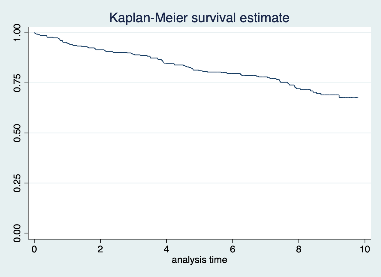
圖 117.1: sts graph, saving(plot1)
117.3 Q3
使用 sts list 命令來查看該數據中第1,3,和5年時的累計生存概率 (cumulative survival probability)。
##
## . cd "~/Downloads/LSHTMlearningnote/backupfile/Users/chaoimacmini/Downloads/LSHTMlearningnote/backupfiles
##
## . use trinmlsh
##
## . quietly stset timeout, fail(death) origin(timein) enter(timein) scale(365.25)
## >  id(id)
##
## . sts list, at(1, 3, 5)
##
##          failure _d:  death
##    analysis time _t:  (timeout-origin)/365.25
##              origin:  time timein
##   enter on or after:  time timein
##                  id:  id
##
##               Beg.                      Survivor      Std.
##     Time     Total     Fail             Function     Error     [95% Conf. Int.]
## -------------------------------------------------------------------------------
##        1       303       16              0.9497    0.0123     0.9192    0.9689
##        3       284       18              0.8930    0.0173     0.8536    0.9224
##        5       256       26              0.8107    0.0220     0.7630    0.8497
## -------------------------------------------------------------------------------
## Note: Survivor function is calculated over full data and evaluated at indicated
##       times; it is not calculated from aggregates shown at left.
##
## .
117.4 Q4
給Q2 的 Kaplan-Meier 曲線添加 95% 信賴區間:
sts graph, ci saving(plot1, replace)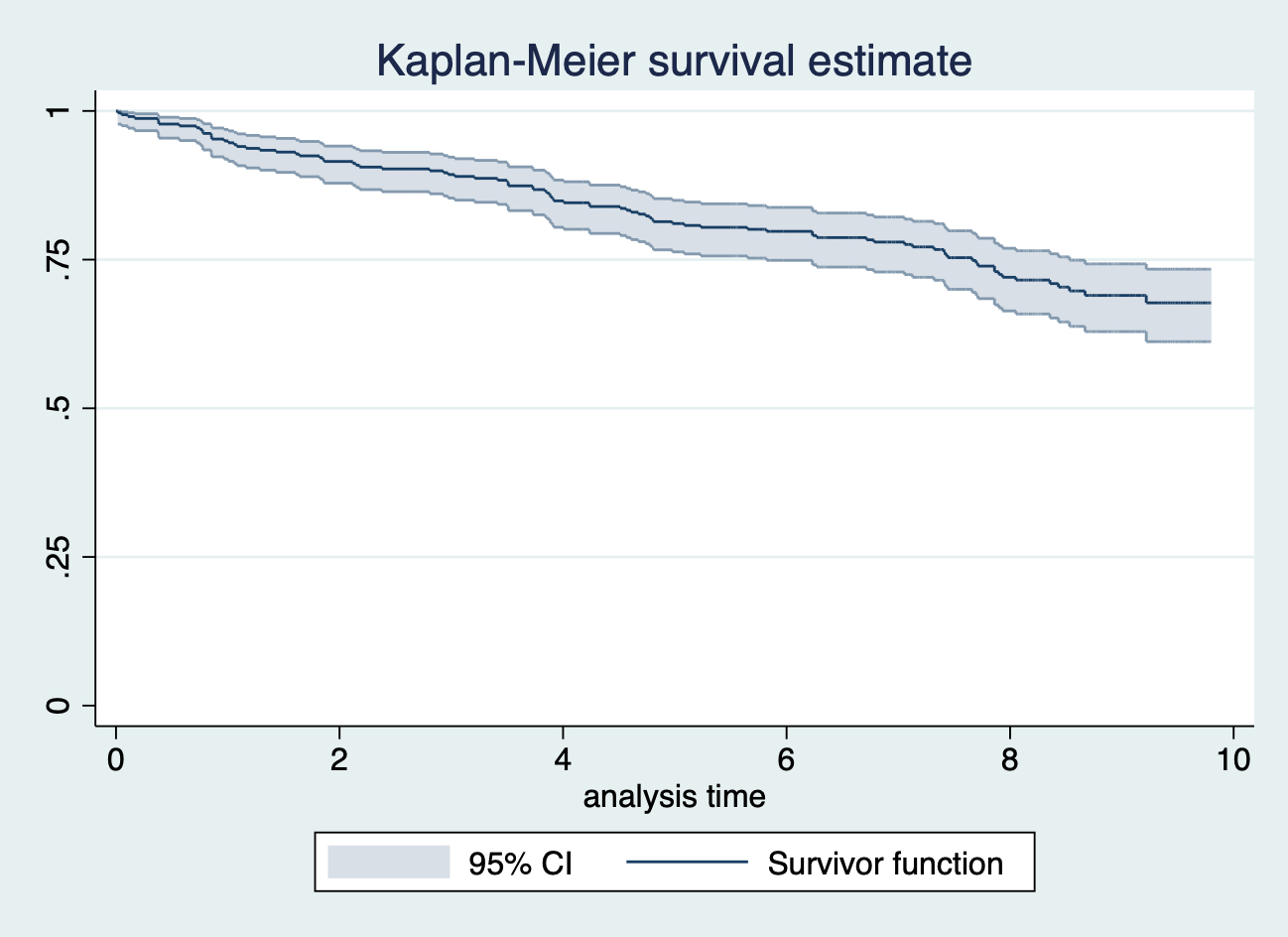
圖 117.2: sts graph, ci saving(plot1, replace)
117.5 Q5
關注變量 smokenum, 查看它的詳細內容。
##
## . cd "~/Downloads/LSHTMlearningnote/backupfile/Users/chaoimacmini/Downloads/LSHTMlearningnote/backupfiles
##
## . use trinmlsh
##
## . quietly stset timeout, fail(death) origin(timein) enter(timein) scale(365.25)
## >  id(id)
##
## . tab smokenum
##
##      No. of |
##  cigarettes |
##     per day |      Freq.     Percent        Cum.
## ------------+-----------------------------------
##    non-smok |        140       44.16       44.16
##    ex-smoke |         68       21.45       65.62
##    1-9 cigs |         29        9.15       74.76
##    10-19 ci |         30        9.46       84.23
##    20-29 ci |         26        8.20       92.43
##    30+ cigs |         24        7.57      100.00
## ------------+-----------------------------------
##       Total |        317      100.00
##
## . tab smokenum, nolabel
##
##      No. of |
##  cigarettes |
##     per day |      Freq.     Percent        Cum.
## ------------+-----------------------------------
##           0 |        140       44.16       44.16
##           1 |         68       21.45       65.62
##           2 |         29        9.15       74.76
##           3 |         30        9.46       84.23
##           4 |         26        8.20       92.43
##           5 |         24        7.57      100.00
## ------------+-----------------------------------
##       Total |        317      100.00
##
## .
生成一個新的變量區分對象是否是現在有吸菸習慣 “current smoker”。比較現在有吸菸習慣和無吸菸習慣的兩組對象的生存曲線,這兩條曲線之間是否有(統計學上的)不同?
##
## . cd "~/Downloads/LSHTMlearningnote/backupfile/Users/chaoimacmini/Downloads/LSHTMlearningnote/backupfiles
##
## . use trinmlsh
##
## . quietly stset timeout, fail(death) origin(timein) enter(timein) scale(365.25)
## >  id(id)
##
## . gen smokstatus = smokenum >= 2 if smokenum != .
## (1 missing value generated)
##
## . label define smokstatus 0 "non-smokers" 1 "current smokers"
##
## . label value smokstatus smokstatus
##
## .
繪製兩組人的生存概率曲線,需要用到 by(smokstatus) 選項。
sts graph, by(smokstatus)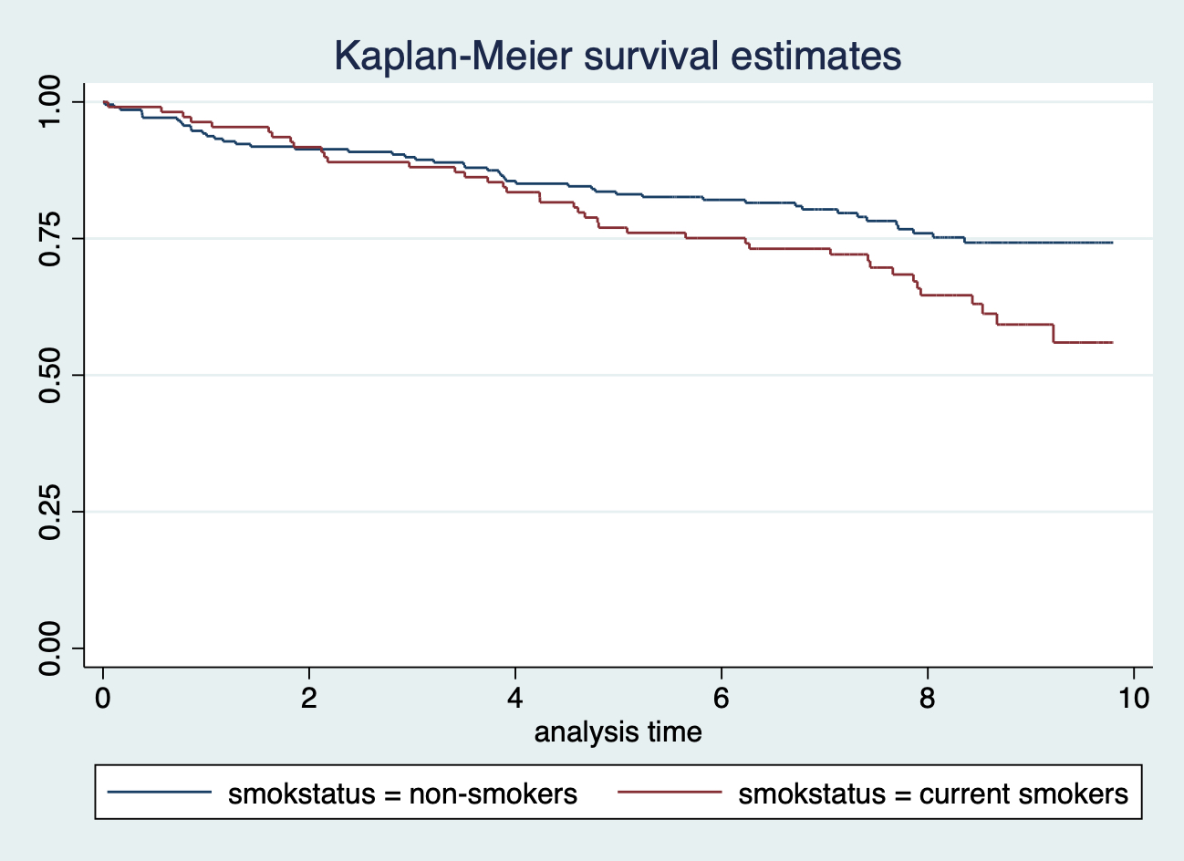
圖 117.3: sts graph, by(smokstatus)
可以看到吸菸和不吸菸兩組人的生存曲線在追蹤到第四年左右之前都十分相似。但是再往後的觀察隨訪時間裏,吸菸者的希望概率似乎要更高。
117.6 Q6
檢驗吸菸習慣不同的兩組實驗對象的生存曲線在整個隨訪過程中是否有統計學意義上的不同?
##
## . cd "~/Downloads/LSHTMlearningnote/backupfile/Users/chaoimacmini/Downloads/LSHTMlearningnote/backupfiles
##
## . use trinmlsh
##
## . quietly stset timeout, fail(death) origin(timein) enter(timein) scale(365.25)
## >  id(id)
##
## . gen smokstatus = smokenum >= 2 if smokenum != .
## (1 missing value generated)
##
## . label define smokstatus 0 "non-smokers" 1 "current smokers"
##
## . label value smokstatus smokstatus
##
## . sts test smokstatus
##
##          failure _d:  death
##    analysis time _t:  (timeout-origin)/365.25
##              origin:  time timein
##   enter on or after:  time timein
##                  id:  id
##
##
## Log-rank test for equality of survivor functions
## ------------------------------------------------
##
##                 |   Events         Events
## smokstatus      |  observed       expected
## ----------------+-------------------------
## non-smokers     |        48          57.86
## current smokers |        40          30.14
## ----------------+-------------------------
## Total           |        88          88.00
##
##                       chi2(1) =       4.91
##                       Pr>chi2 =     0.0267
##
## .
Logrank 檢驗結果提示吸菸和不吸菸兩組人的生存曲線確實存在統計學上的差異 (p = 0.03)。
117.7 Q7
打開 mortality 數據。該隊列研究在北部尼日利亞地區實施了三年。我們主要在這裏觀察分析高血壓和總死亡之間的關係。
##
## . cd "~/Downloads/LSHTMlearningnote/backupfile/Users/chaoimacmini/Downloads/LSHTMlearningnote/backupfiles
##
## . use mortality, clear
##
## . describe
##
## Contains data from mortality.dta
##   obs:         4,298
##  vars:            28                          23 Oct 2013 11:45
## -------------------------------------------------------------------------------
##               storage   display    value
## variable name   type    format     label      variable label
## -------------------------------------------------------------------------------
## id              int     %8.0g                 Individual ID
## area            float   %9.0g      area       Area
## district        str7    %7s                   District
## vcode           byte    %8.0g                 Village ID
## compound_size   float   %9.0g                 Compound size
## age             byte    %8.0g                 Age in years
## sex             byte    %8.0g      sex        Sex
## ethnic          byte    %8.0g      ethnic     Ethnic
## religion        byte    %11.0g     religion   Religion
## occupation      byte    %27.0g     occupation
##                                               Occupation
## education       byte    %22.0g     education
##                                               Education
## mfpermg         float   %9.0g                 Microfilarial load per mg
## vimp            float   %17.0g     vimp       Visually impaired
## died            float   %9.0g                 Died
## systolic        int     %8.0g                 Systolic BP (mmHg)
## diastolic       int     %8.0g                 Diastolic BP (mmHg)
## pulse           int     %8.0g                 Pulse rate/minute
## weight          int     %8.0g                 Weight (kgs)
## height          int     %8.0g                 Height (cms)
## map             float   %9.0g                 Mean Arterial Pressure
## bmi             float   %9.0g                 BMI
## agegrp          float   %9.0g      agegrp     Age group (years)
## mfgrp           float   %10.0g     mfgrp      Microfilarial load/mg (grouped)
## mfpos           float   %9.0g                 Microfilarial infection
## agebin          float   %9.0g      agebin     Age (2 groups)
## bmigrp          float   %12.0g     bmigrp     BMI (3 groups)
## enter           long    %dD_m_Y               Date of entry to study
## exit            float   %dD_m_Y               Date of exit from study
## -------------------------------------------------------------------------------
## Sorted by: id
##
## .
117.8 Q8
使用 gen 命令生成一個新的變量,根據收縮期血壓 (based on systolic blood pressure) 定義實驗對象是否有高血壓。
##
## . cd "~/Downloads/LSHTMlearningnote/backupfile/Users/chaoimacmini/Downloads/LSHTMlearningnote/backupfiles
##
## . use mortality, clear
##
## . gen hyper = .
## (4,298 missing values generated)
##
## . replace hyper = 0 if systolic < 140
## (3,747 real changes made)
##
## . replace hyper = 1 if systolic >= 140 & systolic != .
## (516 real changes made)
##
## .
117.9 Q9
使用 stset 命令準備你的數據,讓它可以在 Stata 裏實施生存分析。
##
## . cd "~/Downloads/LSHTMlearningnote/backupfile/Users/chaoimacmini/Downloads/LSHTMlearningnote/backupfiles
##
## . use mortality, clear
##
## . stset exit, failure(died) enter(enter) origin(enter) id(id) scale(365.25)
##
##                 id:  id
##      failure event:  died != 0 & died < .
## obs. time interval:  (exit[_n-1], exit]
##  enter on or after:  time enter
##  exit on or before:  failure
##     t for analysis:  (time-origin)/365.25
##             origin:  time enter
##
## ------------------------------------------------------------------------------
##       4,298  total observations
##           0  exclusions
## ------------------------------------------------------------------------------
##       4,298  observations remaining, representing
##       4,298  subjects
##         137  failures in single-failure-per-subject data
##  11,457.357  total analysis time at risk and under observation
##                                                 at risk from t =         0
##                                      earliest observed entry t =         0
##                                           last observed exit t =  3.249829
##
## .
117.10 Q10
使用 strate 命令計算有高血壓和無高血壓兩組人個字的總死亡率 all-cause mortality rate。
##
## . cd "~/Downloads/LSHTMlearningnote/backupfile/Users/chaoimacmini/Downloads/LSHTMlearningnote/backupfiles
##
## . use mortality, clear
##
## . gen hyper = .
## (4,298 missing values generated)
##
## . quietly replace hyper = 0 if systolic < 140
##
## . quietly replace hyper = 1 if systolic >= 140 & systolic != .
##
## . quietly stset exit, failure(died) enter(enter) origin(enter) id(id) scale(365
## > .25)
##
## . strate hyper, per(1000)
##
##          failure _d:  died
##    analysis time _t:  (exit-origin)/365.25
##              origin:  time enter
##   enter on or after:  time enter
##                  id:  id
##
## Estimated failure rates
## Number of records  =       4263
##
##   +---------------------------------------------------+
##   | hyper    D        Y      Rate     Lower     Upper |
##   |---------------------------------------------------|
##   |     0   94   9.9879    9.4114    7.6888   11.5199 |
##   |     1   40   1.3819   28.9456   21.2322   39.4611 |
##   +---------------------------------------------------+
##    Notes: Rate = D/Y = failures/person-time (per 1000).
##           Lower and Upper are bounds of 95% confidence intervals.
##
##
## .
計算結果是高血壓的實驗對象中,總死亡率達到每 1000 人年 28.95,沒有高血壓的人羣的死亡率是9.4 每 1000人年。
117.11 Q11
使用 stmh 命令計算高血壓和總死亡之間的關係,比較有高血壓的人相對無高血壓人的總體死亡率比 rate ratio。
##
## . cd "~/Downloads/LSHTMlearningnote/backupfile/Users/chaoimacmini/Downloads/LSHTMlearningnote/backupfiles
##
## . use mortality, clear
##
## . gen hyper = .
## (4,298 missing values generated)
##
## . quietly replace hyper = 0 if systolic < 140
##
## . quietly replace hyper = 1 if systolic >= 140 & systolic != .
##
## . quietly stset exit, failure(died) enter(enter) origin(enter) id(id) scale(365
## > .25)
##
## . stmh hyper
##
##          failure _d:  died
##    analysis time _t:  (exit-origin)/365.25
##              origin:  time enter
##   enter on or after:  time enter
##                  id:  id
##
## Mantel-Haenszel estimate of the rate ratio
##   comparing hyper==1 vs. hyper==0
##
## ------------------------------------------------------------------------
##     Rate ratio         chi2         P>chi2          [95% Conf. Interval]
## ------------------------------------------------------------------------
##          3.076        39.30         0.0000              2.124      4.453
## ------------------------------------------------------------------------
##
## .
計算死亡率比的結果表示,有高血壓的實驗對象色死亡率是無高血壓的人死亡率的三倍還多。
117.12 Q12-13
這時候,我們使用 browse 瀏覽正在分析的數據時,會發現最後幾個新增的變量。
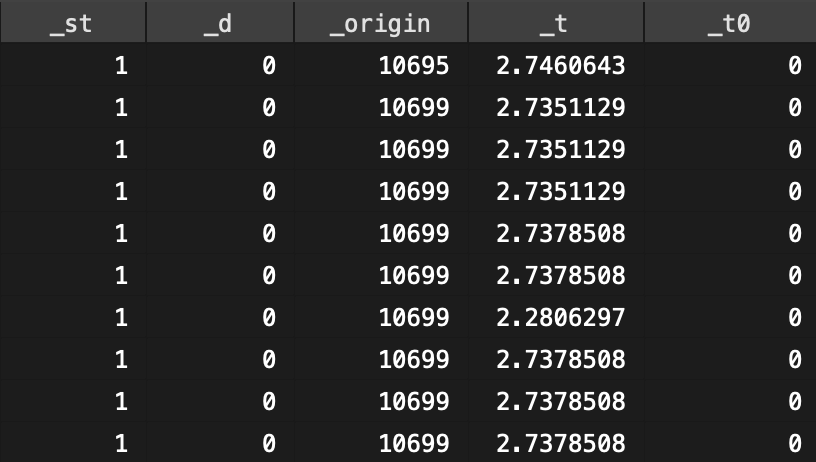
圖 117.4: New variables generated by Stata to calcuate rate.(1)
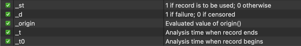
圖 117.5: New variables generated by Stata to calcuate rate.(2)
新增的幾個變量分別定義爲:
_st is an indicator variable taking the value 0 or 1. 1 indicates records included in the analyses, 0 indicates records excluded from analyses, for example if the exit time was earlier than the entry time

_d records whether the individual experienced the event (=1) or not (=0). In this simple situation _d = died (try tab _d died)

_t is the time the person exited the study (in years since entry to the study)

_t0 is the time the person entered the study (in years since entry to the study, so zero for everyone)
117.13 Q14
製作一個生存表格,只保留高血壓人羣。
##
## . cd "~/Downloads/LSHTMlearningnote/backupfile/Users/chaoimacmini/Downloads/LSHTMlearningnote/backupfiles
##
## . use mortality, clear
##
## . gen hyper = .
## (4,298 missing values generated)
##
## . quietly replace hyper = 0 if systolic < 140
##
## . quietly replace hyper = 1 if systolic >= 140 & systolic != .
##
## . quietly stset exit, failure(died) enter(enter) origin(enter) id(id) scale(365
## > .25)
##
## . sts list if hyper == 1
##
##          failure _d:  died
##    analysis time _t:  (exit-origin)/365.25
##              origin:  time enter
##   enter on or after:  time enter
##                  id:  id
##
##              At           Net    Survivor      Std.
##   Time     Risk   Fail   Lost    Function     Error     [95% Conf. Int.]
## ------------------------------------------------------------------------
##    .23      516      1      0      0.9981    0.0019     0.9863    0.9997
##  .2533      515      1      0      0.9961    0.0027     0.9846    0.9990
##  .3559      514      1      0      0.9942    0.0033     0.9821    0.9981
##  .3587      513      0      1      0.9942    0.0033     0.9821    0.9981
##  .3669      512      0      1      0.9942    0.0033     0.9821    0.9981
##  .3723      511      1      0      0.9922    0.0039     0.9795    0.9971
##  .3792      510      1      0      0.9903    0.0043     0.9768    0.9959
##  .3888      509      1      0      0.9883    0.0047     0.9743    0.9947
##  .4298      508      1      0      0.9864    0.0051     0.9717    0.9935
##  .4353      507      0      1      0.9864    0.0051     0.9717    0.9935
##  .4408      506      1      0      0.9845    0.0055     0.9692    0.9922
##  .4846      505      2      0      0.9806    0.0061     0.9642    0.9895
##  .5421      503      0      1      0.9806    0.0061     0.9642    0.9895
##  .6886      502      0      1      0.9806    0.0061     0.9642    0.9895
##  .8378      501      0      1      0.9806    0.0061     0.9642    0.9895
##  .9363      500      0      1      0.9806    0.0061     0.9642    0.9895
##  .9514      499      0      1      0.9806    0.0061     0.9642    0.9895
##  1.003      498      1      0      0.9786    0.0064     0.9617    0.9881
##  1.012      497      0      1      0.9786    0.0064     0.9617    0.9881
##  1.016      496      1      0      0.9766    0.0067     0.9592    0.9867
##  1.047      495      1      0      0.9746    0.0069     0.9567    0.9852
##   1.05      494      1      0      0.9727    0.0072     0.9543    0.9837
##  1.055      493      0      1      0.9727    0.0072     0.9543    0.9837
##  1.336      492      1      0      0.9707    0.0075     0.9519    0.9822
##  1.377      491      1      0      0.9687    0.0077     0.9494    0.9807
##  1.399      490      1      0      0.9667    0.0079     0.9470    0.9792
##  1.418      489      0      1      0.9667    0.0079     0.9470    0.9792
##  1.425      488      2      0      0.9628    0.0084     0.9423    0.9761
##  1.477      486      0      1      0.9628    0.0084     0.9423    0.9761
##  1.569      485      1      0      0.9608    0.0086     0.9399    0.9745
##  1.574      484      1      0      0.9588    0.0088     0.9375    0.9729
##  1.585      483      1      0      0.9568    0.0090     0.9352    0.9714
##  1.619      482      1      0      0.9548    0.0092     0.9328    0.9698
##  1.941      481      1      1      0.9528    0.0094     0.9305    0.9681
##  2.029      479      1      0      0.9509    0.0096     0.9281    0.9665
##   2.04      478      1      0      0.9489    0.0098     0.9258    0.9649
##  2.277      477      0      1      0.9489    0.0098     0.9258    0.9649
##  2.286      476      0      1      0.9489    0.0098     0.9258    0.9649
##  2.289      475      1      0      0.9469    0.0100     0.9235    0.9633
##  2.311      474      0      2      0.9469    0.0100     0.9235    0.9633
##  2.313      472      0      3      0.9469    0.0100     0.9235    0.9633
##  2.316      469      0      2      0.9469    0.0100     0.9235    0.9633
##  2.319      467      0      5      0.9469    0.0100     0.9235    0.9633
##  2.322      462      0      2      0.9469    0.0100     0.9235    0.9633
##  2.326      460      1      0      0.9448    0.0101     0.9211    0.9616
##  2.404      459      0      1      0.9448    0.0101     0.9211    0.9616
##  2.407      458      0      2      0.9448    0.0101     0.9211    0.9616
##  2.409      456      0      3      0.9448    0.0101     0.9211    0.9616
##  2.412      453      0      7      0.9448    0.0101     0.9211    0.9616
##  2.415      446      0      4      0.9448    0.0101     0.9211    0.9616
##  2.416      442      1      0      0.9427    0.0103     0.9185    0.9598
##  2.439      441      0      3      0.9427    0.0103     0.9185    0.9598
##  2.442      438      0      2      0.9427    0.0103     0.9185    0.9598
##  2.445      436      0      5      0.9427    0.0103     0.9185    0.9598
##  2.448      431      0      3      0.9427    0.0103     0.9185    0.9598
##   2.45      428      0      2      0.9427    0.0103     0.9185    0.9598
##  2.453      426      0      5      0.9427    0.0103     0.9185    0.9598
##  2.471      421      1      0      0.9404    0.0106     0.9159    0.9580
##  2.472      420      1      0      0.9382    0.0108     0.9132    0.9561
##  2.478      419      1      0      0.9360    0.0110     0.9106    0.9543
##   2.48      418      0      4      0.9360    0.0110     0.9106    0.9543
##  2.483      414      0      3      0.9360    0.0110     0.9106    0.9543
##  2.486      411      0      9      0.9360    0.0110     0.9106    0.9543
##  2.489      402      0     14      0.9360    0.0110     0.9106    0.9543
##   2.49      388      0      1      0.9360    0.0110     0.9106    0.9543
##  2.491      387      2      8      0.9311    0.0114     0.9048    0.9503
##  2.494      377      1      7      0.9287    0.0117     0.9019    0.9483
##  2.497      369      1      3      0.9261    0.0119     0.8989    0.9462
##    2.5      365      0      5      0.9261    0.0119     0.8989    0.9462
##  2.502      360      0      2      0.9261    0.0119     0.8989    0.9462
##  2.505      358      0      3      0.9261    0.0119     0.8989    0.9462
##  2.639      355      0      2      0.9261    0.0119     0.8989    0.9462
##  2.642      353      0      8      0.9261    0.0119     0.8989    0.9462
##  2.645      345      0      8      0.9261    0.0119     0.8989    0.9462
##  2.648      337      1      7      0.9234    0.0122     0.8956    0.9440
##   2.65      329      0      6      0.9234    0.0122     0.8956    0.9440
##  2.653      323      0      6      0.9234    0.0122     0.8956    0.9440
##  2.656      317      0      8      0.9234    0.0122     0.8956    0.9440
##  2.667      309      0      1      0.9234    0.0122     0.8956    0.9440
##   2.68      308      0      1      0.9234    0.0122     0.8956    0.9440
##  2.682      307      1      1      0.9204    0.0125     0.8919    0.9416
##  2.684      305      1      0      0.9174    0.0128     0.8882    0.9392
##  2.715      304      1      0      0.9143    0.0131     0.8846    0.9367
##  2.719      303      0      1      0.9143    0.0131     0.8846    0.9367
##  2.721      302      0      1      0.9143    0.0131     0.8846    0.9367
##  2.727      301      0      3      0.9143    0.0131     0.8846    0.9367
##   2.73      298      0     14      0.9143    0.0131     0.8846    0.9367
##  2.732      284      0      6      0.9143    0.0131     0.8846    0.9367
##  2.735      278      0      4      0.9143    0.0131     0.8846    0.9367
##  2.738      274      0      4      0.9143    0.0131     0.8846    0.9367
##  2.741      270      0     13      0.9143    0.0131     0.8846    0.9367
##  2.743      257      0      4      0.9143    0.0131     0.8846    0.9367
##  2.746      253      0      5      0.9143    0.0131     0.8846    0.9367
##  2.757      248      0      1      0.9143    0.0131     0.8846    0.9367
##  2.793      247      0      1      0.9143    0.0131     0.8846    0.9367
##  2.812      246      0      1      0.9143    0.0131     0.8846    0.9367
##  2.815      245      0      7      0.9143    0.0131     0.8846    0.9367
##  2.817      238      0      3      0.9143    0.0131     0.8846    0.9367
##  2.823      235      0      2      0.9143    0.0131     0.8846    0.9367
##  2.825      233      0      4      0.9143    0.0131     0.8846    0.9367
##  2.828      229      0      4      0.9143    0.0131     0.8846    0.9367
##  2.831      225      0      3      0.9143    0.0131     0.8846    0.9367
##  2.834      222      0      1      0.9143    0.0131     0.8846    0.9367
##  2.875      221      0      2      0.9143    0.0131     0.8846    0.9367
##  2.899      219      0      1      0.9143    0.0131     0.8846    0.9367
##  2.962      218      0      1      0.9143    0.0131     0.8846    0.9367
##  2.965      217      0      8      0.9143    0.0131     0.8846    0.9367
##  2.968      209      0      7      0.9143    0.0131     0.8846    0.9367
##  2.971      202      0      9      0.9143    0.0131     0.8846    0.9367
##  2.973      193      0     20      0.9143    0.0131     0.8846    0.9367
##  2.976      173      0      8      0.9143    0.0131     0.8846    0.9367
##  2.979      165      0      5      0.9143    0.0131     0.8846    0.9367
##  2.982      160      0      3      0.9143    0.0131     0.8846    0.9367
##  2.984      157      0      3      0.9143    0.0131     0.8846    0.9367
##   2.99      154      0      2      0.9143    0.0131     0.8846    0.9367
##  2.995      152      0      1      0.9143    0.0131     0.8846    0.9367
##  3.001      151      0      1      0.9143    0.0131     0.8846    0.9367
##  3.039      150      0      4      0.9143    0.0131     0.8846    0.9367
##  3.042      146      0      2      0.9143    0.0131     0.8846    0.9367
##  3.044      144      0      3      0.9143    0.0131     0.8846    0.9367
##  3.047      141      0      4      0.9143    0.0131     0.8846    0.9367
##   3.05      137      0      2      0.9143    0.0131     0.8846    0.9367
##  3.053      135      0      3      0.9143    0.0131     0.8846    0.9367
##  3.061      132      0      1      0.9143    0.0131     0.8846    0.9367
##  3.072      131      0      2      0.9143    0.0131     0.8846    0.9367
##   3.08      129      0      7      0.9143    0.0131     0.8846    0.9367
##  3.083      122      0      4      0.9143    0.0131     0.8846    0.9367
##  3.086      118      0      3      0.9143    0.0131     0.8846    0.9367
##  3.088      115      0      3      0.9143    0.0131     0.8846    0.9367
##  3.091      112      0      1      0.9143    0.0131     0.8846    0.9367
##  3.113      111      0      1      0.9143    0.0131     0.8846    0.9367
##  3.116      110      0      6      0.9143    0.0131     0.8846    0.9367
##  3.118      104      0     12      0.9143    0.0131     0.8846    0.9367
##  3.121       92      0      8      0.9143    0.0131     0.8846    0.9367
##  3.143       84      0      1      0.9143    0.0131     0.8846    0.9367
##  3.146       83      0      8      0.9143    0.0131     0.8846    0.9367
##  3.149       75      0     13      0.9143    0.0131     0.8846    0.9367
##  3.151       62      0     19      0.9143    0.0131     0.8846    0.9367
##  3.157       43      0      1      0.9143    0.0131     0.8846    0.9367
##  3.159       42      0      4      0.9143    0.0131     0.8846    0.9367
##  3.162       38      0      8      0.9143    0.0131     0.8846    0.9367
##  3.165       30      0     15      0.9143    0.0131     0.8846    0.9367
##  3.168       15      0     10      0.9143    0.0131     0.8846    0.9367
##   3.17        5      0      4      0.9143    0.0131     0.8846    0.9367
## ------------------------------------------------------------------------
## Note: Net Lost equals the number lost minus the number who entered.
##
## .
117.16 Q17
Kaplan Meier 生存曲線繪製的是累計生存概率,我們再來嘗試繪製累計死亡率,
sts graph, by(hyper) ci failure ylabel(0 0.05 0.10 0.15 0.20)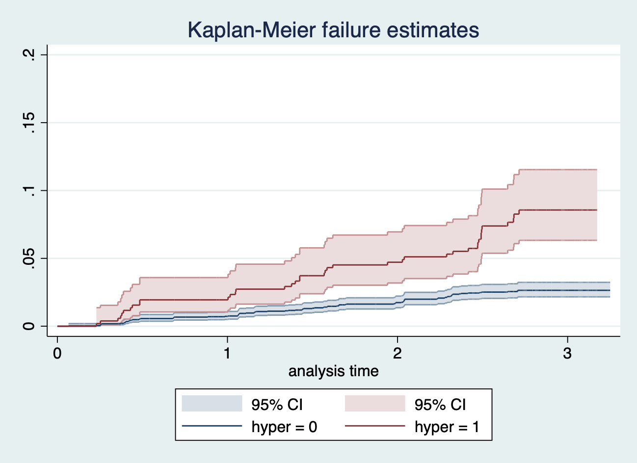
圖 117.8: sts graph, by(hyper) ci failure ylabel(0 0.05 0.10 0.15 0.20)
117.17 Q18
使用 Logrank 檢驗法檢驗有無高血壓之間是否存在統計學上的生存曲線差異。
##
## . cd "~/Downloads/LSHTMlearningnote/backupfile/Users/chaoimacmini/Downloads/LSHTMlearningnote/backupfiles
##
## . use mortality, clear
##
## . gen hyper = .
## (4,298 missing values generated)
##
## . quietly replace hyper = 0 if systolic < 140
##
## . quietly replace hyper = 1 if systolic >= 140 & systolic != .
##
## . quietly stset exit, failure(died) enter(enter) origin(enter) id(id) scale(365
## > .25)
##
## . sts test hyper
##
##          failure _d:  died
##    analysis time _t:  (exit-origin)/365.25
##              origin:  time enter
##   enter on or after:  time enter
##                  id:  id
##
##
## Log-rank test for equality of survivor functions
## ------------------------------------------------
##
##       |   Events         Events
## hyper |  observed       expected
## ------+-------------------------
## 0     |        94         117.91
## 1     |        40          16.09
## ------+-------------------------
## Total |       134         134.00
##
##             chi2(1) =      40.36
##             Pr>chi2 =     0.0000
##
## .
我們發現數據提供了極強的證據證明有無高血壓人羣之間確實是存在生存曲線的統計學差異。
117.18 Q19
這次我們重新使用 stset 命令來準備生存數據,但是我們不指定時間的起點 origin:
##
## . cd "~/Downloads/LSHTMlearningnote/backupfile/Users/chaoimacmini/Downloads/LSHTMlearningnote/backupfiles
##
## . use mortality, clear
##
## . stset exit, failure(died) enter(enter) id(id) scale(365.25)
##
##                 id:  id
##      failure event:  died != 0 & died < .
## obs. time interval:  (exit[_n-1], exit]
##  enter on or after:  time enter
##  exit on or before:  failure
##     t for analysis:  time/365.25
##
## ------------------------------------------------------------------------------
##       4,298  total observations
##           0  exclusions
## ------------------------------------------------------------------------------
##       4,298  observations remaining, representing
##       4,298  subjects
##         137  failures in single-failure-per-subject data
##  11,457.357  total analysis time at risk and under observation
##                                                 at risk from t =         0
##                                      earliest observed entry t =  28.94182
##                                           last observed exit t =  32.21355
##
## .
此時,這個數據中因這一行命令產生的新變量 _t 其實是每個實驗對象從時間點 1960/01/01 到他們各自離開實驗追蹤的時間長度。而 _t0 則是每個實驗對象從時間點 1960/01/01 到他們各自參加這個實驗的時間長度。當我們使用 strate 和 stmh 來評價高血壓和死亡之間的關係的時候會得到和之前相同的分析結果。
##
## . cd "~/Downloads/LSHTMlearningnote/backupfile/Users/chaoimacmini/Downloads/LSHTMlearningnote/backupfiles
##
## . use mortality, clear
##
## . gen hyper = .
## (4,298 missing values generated)
##
## . quietly replace hyper = 0 if systolic < 140
##
## . quietly replace hyper = 1 if systolic >= 140 & systolic != .
##
## . quietly stset exit, failure(died) enter(enter) id(id) scale(365.25)
##
## . strate hyper, per(1000)
##
## failure _d: died
## analysis time _t: exit/365.25
## enter on or after: time enter
## id: id
##
## Estimated failure rates
## Number of records = 4263
##
## +---------------------------------------------------+
## | hyper D Y Rate Lower Upper |
## |---------------------------------------------------|
## | 0 94 9.9879 9.4114 7.6888 11.5199 |
## | 1 40 1.3819 28.9456 21.2322 39.4611 |
## +---------------------------------------------------+
## Notes: Rate = D/Y = failures/person-time (per 1000).
## Lower and Upper are bounds of 95% confidence intervals.
##
##
## . stmh hyper
##
## failure _d: died
## analysis time _t: exit/365.25
## enter on or after: time enter
## id: id
##
## Mantel-Haenszel estimate of the rate ratio
## comparing hyper==1 vs. hyper==0
##
## ------------------------------------------------------------------------
## Rate ratio chi2 P>chi2 [95% Conf. Interval]
## ------------------------------------------------------------------------
## 3.076 39.30 0.0000 2.124 4.453
## ------------------------------------------------------------------------
##
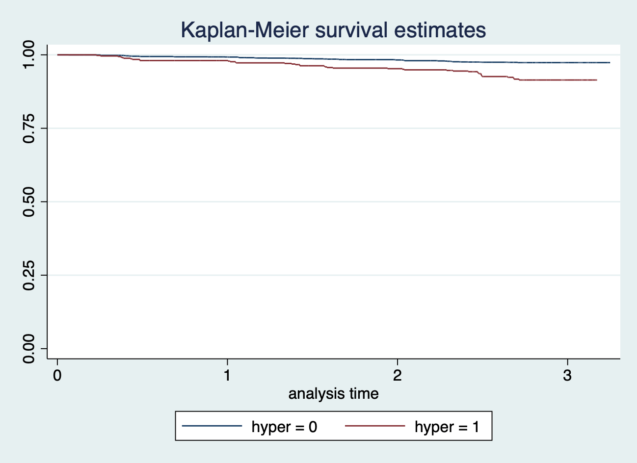
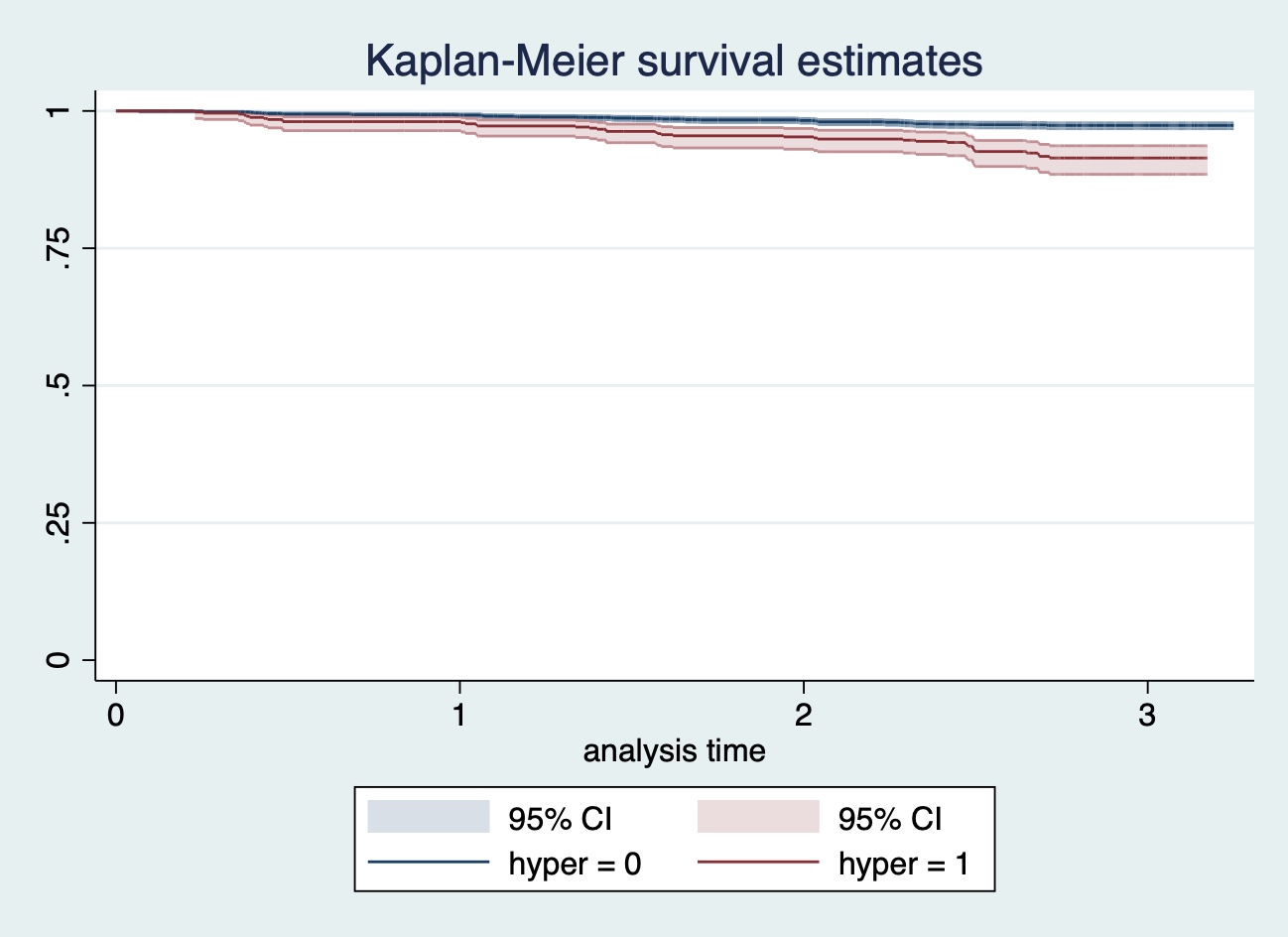
## .那現在繪製的 Kaplan-Meier 生存曲線會變成什麼樣子呢?
sts graph, by(hyper)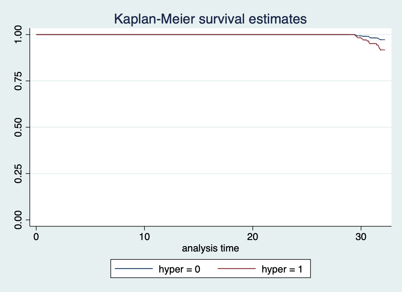
圖 117.9: sts graph, by(hyper) without specifying origin in stset command.
所以,當我們忘記設定實驗的起點時間 origin 時,Stata自動把所有實驗的時間起點設置成 1960/01/01。