第 97 章 共軛先驗概率 Conjugate priors
本章節我們重溫一下最早在貝葉斯統計學入門部分(Chapter 41)介紹過的一些基本原則。特別是關於共軛先驗概率的概念,並提供一些使用BUGS模型的例子來展示如何運算這些模型。
97.1 貝葉斯推斷的基礎
在一個臨牀試驗中,作爲一名貝葉斯統計學者,必須清晰明瞭地闡述如下幾個問題:
- 合理地描述目前爲止,在瞭解本次試驗數據的結果之前,類似研究曾經給出過的療效差異的報告結果,可能的取值範圍 (the prior distribution);
- 本次試驗數據得到的結果,支持怎樣的療效差異 (the likelihood);
之後需要將上述兩個資源通過合理的數學模型結合在一起,用於產生 - 最終療效是否存在的意見和建議,證據的總結 (the posterior distribution)。
最後第三步將先驗概率和似然相結合的過程,用到的是貝葉斯定理(Bayes Theorem)。通過貝葉斯定理把目前位置的經驗作爲先驗概率統合現階段試驗數據給出的似然的過程,其實是一個自我學習不斷更新知識的過程。經過貝葉斯推斷,給出事後概率分布之時,我們可以拿它來做什麼呢?
- 估計和評價治療效果,治療差異。
- 估計和評價模型中參數的不確定性。
- 計算你感興趣的那個變量(可以是療效差異,可以是模型中的參數)達到或者超過某個特定目標值的概率。
- 預測你感興趣的那個變量可能存在的範圍。
- 作爲未來要進行的試驗設計階段的先驗概率分布。
- 給決策者提供證據。
你是否還記得貝葉斯定理的公式: 如果\(A, B\)分別標記兩個事件,那麼有
\[ p(A|B) = \frac{p(B|A)p(A)}{p(B)} \]
如果\(A_i\)是一系列互斥不相交事件,也就是\(p(\cup_iA_i) = \sum_ip(A_i) = 1\),貝葉斯定理可以被改寫成爲:
\[ p(A_i|B) = \frac{p(B|A_i)p(A_i)}{\sum_jp(B|A_j)p(A_j)} \]
貝葉斯統計學推斷從根本上的特點在於嚴格區分:
- 觀測數據 \(y\),也就是試驗獲得的數據。
- 未知參數 \(\theta\),這裏,\(\theta\)可以用統計學工具來描述,它可以是統計學參數,可以是缺失值,可以是測量誤差數據等等。
- 這裏貝葉斯統計學把未知參數當做一個可以變化的隨機變量(parameters are treated as random variables);
- 在貝葉斯統計學框架下,我們對參數的不確定性進行描述(we make probability statements about model parameters)。
- 在概率論統計學框架下,統計學參數是未知,但是確實不變的。使用概率論統計學進行推斷時,我們只對數據進行不確定性的描述(parameters are fixed non-random quantities and the probability statements concern the data.)
貝葉斯統計學推斷中,我們仍然需要建立模型用來描述 \(p(y|\theta)\),這個也就是概率論統計學中常見的似然(likelihood)。似然是把各個變量關聯起來的完整的概率模型(full probability model)。
從貝葉斯統計學推斷的觀點出發,
- 在實施試驗,收集數據之前,參數(\(\theta\))是未知的,所以它需要由一個概率分布(probability distribution)來反應它的不確定性,也就是說,我們需要先對參數可能來自的分布進行描述,指定一個先驗概率(prior distribution)\(p(\theta)\);
- 試驗進行完了,數據整理分析之時,我們知道了\(y\),這就是我們來和先驗概率結合的似然,使用貝葉斯定理,從而獲得給定了觀測數據之後(conditional on),服從先驗概率的參數現在服從的概率分布,這被叫做事後概率分布(posterior distribution)。
\[ p(\theta|y) = \frac{p(\theta)p(y|\theta)}{\int p(\theta)p(y|\theta)d\theta} \propto p(\theta)p(y|\theta) \]
總結一下就是,
- 先驗概率(prior distribution),\(p(\theta)\)描述的是在收集數據之前參數的不確定性。
- 事後概率(posterior distribution),\(p(\theta | y)\) 描述的是在收集數據之後參數的不確定性。
97.2 二項分布(似然)數據的共軛先驗概率
沿用前一個章節新藥試驗的例子。我們在實施試驗之前對藥物的認知是,我們認爲它的藥效概率可能在 0.2-0.6 之間。我們把這個試驗前對藥物療效的估計認知翻譯成一個服從均值爲0.4,標準差爲0.1的Beta分布。這個Beta分布使用的參數(參數的參數被叫做超參數, hyperparameter),是9.2, 13.8,寫作\(\text{Beta}(9.2, 13.8)\)。那麼現在我們假設試驗結束,收集的20名患者中15名療效顯著。接下來貝葉斯統計學家要回答的問題是,這個試驗結果對先驗概率分布產生了多大的影響(How should this trial change our opinion about the positive response rate)?
在這個例子中,我們現在來詳細給出先驗概率和似然。
- 似然 likelihood (distribution of the data):
如果患者可以被認爲是相互獨立的,他們來自一個相同的總體,在這個總體中有一個未知的對藥物療效有效反應(positive response)的概率 \(\theta\),這樣的數據可以用一個二項分布似然來描述 binomial likelihood:
\[ p(y | n, \theta) = \binom{n}{y}\theta^y(1-\theta)^{n-y} \propto \theta^y(1-\theta)^{n-y} \]
- 描述試驗前我們對\(\theta\)的認知的先驗概率 prior distribution,這是一個連續型先驗概率分布。
對於百分比,我們用Beta分布來描述:
\[ \begin{aligned} \theta & \sim \text{Beta}(a,b) \\ p(\theta) & = \frac{\Gamma(a+b)}{\Gamma(a)\Gamma(b)} \theta^{a-1}(1-\theta)^{b-1}\\ \end{aligned} \]
根據貝葉斯定理,我們來把先驗概率分布和似然相結合(相乘),來獲取事後概率分布:
\[ \begin{aligned} p(\theta | y, n) & \propto p(y|\theta, n)p(\theta) \\ & \propto \theta^y(1-\theta)^{n-y}\theta^{a-1}(1-\theta)^{b-1} \\ & = \theta^{y + a -1}(1-\theta)^{n - y + b -1} \end{aligned} \] 眼尖的人立刻能看出來,這個事後概率分布本身也是一個Beta分布的概率方程,只是它的超參數和先驗概率相比發生了變化(更新):
\[ p(\theta | y,n) = \text{Beta}(a + y, b + n -y) \]
像這樣,先驗概率和事後概率兩個概率分布都來自相同分佈家族的情況,先驗概率又被叫做和似然成共軛關系的先驗概率(共軛先驗概率, conjugate prior)。
par(mfrow=c(3,1))
# Plot exact prior probability density
# values of the hyperparameters
a <- 9.2
b <- 13.8

# prior function
prior <- Vectorize(function(theta) dbeta(theta, a, b))
# Plot
curve(prior, 0, 1, type = "l", main = "Prior for "~theta, ylim = c(0, 4.5), frame = F,
      xlab = "Probability of positive response", ylab = "Density", lwd = 2, cex.axis = 1.5, cex.lab = 1.5)

# binomial likelihood function (likelihood)

Likelihood <- Vectorize(function(theta) dbinom(15, 20, theta))

# Plot
curve(Likelihood, 0, 1, type = "l", main = "Likelihood for the data",
      frame = FALSE, xlab = "Probability of positive response", ylab = "Density",
      lwd = 2, cex.axis =  1.5, cex.lab = 1.5)
# n <- 0; r <- 0; a <- 9.2; b <- 13.8; np <- 20
# plot(0:20, BetaBinom(0:20), type = "b", xlab = "r*", ylab = "P(R = r*)",
#      main = "Prior predictive: a = 9.2, b = 13.8")

# Posterior function

posterior <- Vectorize(function(theta) dbeta(theta, a+15, b+20-15))

# Plot

curve(posterior, 0, 1, type = "l", main = "Posterior for "~theta,
      frame = FALSE, xlab = "Probability of positive response", ylab = "Density",
      lwd = 2, cex.axis = 1.5, cex.lab = 1.5)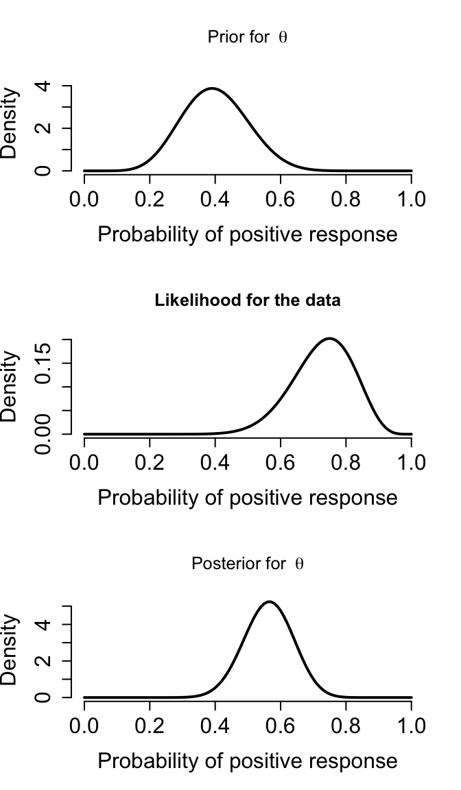
圖 97.1: Prior, likelihood, and posterior for Drug example
本次試驗的模型,它的三個部分(先驗概率,似然,事後概率),分別從上到下繪制在圖 97.1 中。由於我們使用了共軛先驗概率,所以我們也可以通過數學的計算(甚至不需要計算機的輔助)也能算出事後概率分布。可是,並不是所有的模型都有共軛先驗概率分布供我們選擇,這時候,蒙特卡羅模擬試驗的算法就提供了強有力的工具。在BUGS/JAGS語言中,我們可以用蒙特卡羅算法,忽視掉那些無法在數學上推導出事後概率分布方程的模型。BUGS本身很厲害,它可以自動識別出我們給它的先驗概率分布是否和似然之間是共軛的,如果是,那麼它會計算出共軛的事後概率分布方程,然後從事後概率分布方程中選取蒙特卡羅樣本。這個新藥試驗的BUGS模型可以寫作:
#  Monte Carlo model for Drug example

model{
    theta   ~ dbeta(9.2,13.8)          # prior distribution
    y       ~ dbin(theta,20)           # sampling distribution (likelihood)
    y       <- 15                      # data
}
你可以看到這個模型和我們在前一章做預測的模型只有第三行指令發生了變化。當時我們是打算要來做試驗結果的預測。此時,我們試驗完畢,觀察到15名患者的疼痛症狀得到了改善,所以試驗數據是15。BUGS/JAGS本身會自動識別出我們是否給似然增加了觀察數據。當它識別到我們不是用這個模型做結果預測時,它會自動明白並且切換到事後概率分布的計算。這個在似然裏面的數據,是它要拿來放到模型中做條件的(observed values, i.e. data needs to be conditioned on)。
97.2.1 事後概率分布預測
假如這個新藥的效果仍然無法讓人覺得信服,我們考慮再做一次試驗徵集更多的患者,如果在這個試驗中,40名患者中有25名或者更多的患者症狀得到緩解,可以考慮把該藥物加入下一次發展計劃當中。這時候,又一次回到了預測概率的問題上來,我們想知道,“再做40人的試驗時,有25名或者更多的患者的症狀可以得到緩解”這件事可能發生的概率。這時候的模型可以被擴展如下:
\[ \begin{split} \theta & \sim \text{Beta}(a,b) & \text{ Prior distribution} \\ y & \sim \text{Binomial}(\theta, n) & \text{ Sampling distribution} \\ y_{\text{pred}} & \sim \text{Binomial}(\theta, m) & \text{ Predictive distribution} \\ P_{\text{crit}} & \sim P(y_{\text{pred}} \geqslant m_{\text{crit}}) & \text{ Probability of exceeding critical threshold} \end{split} \]
這段模型翻譯成BUGS語言可以描述爲:
model{
  theta     ~ dbeta(a, b)                  # prior distribution
  y         ~ dbin(theta, n)               # sampling distribution
  y.pred    ~ dbin(theta, m)               # predictive distribution
  P.crit   <- step(y.pred - mcrit + 0.5)   # = 1 if y.pred >= mcrit, 0 otherwise
}
我們可以把數據寫在另一個txt文件/向量裏面:
list(a = 9.2,             # parameters of prior distribution
     b = 13.8,
     y = 15,              # number of successes in completed trial
     n = 20,              # number of patients in completed trial
     m = 40,              # number of patients in future trial
     mcrit = 25)          # critical value of future successes
當然這是一個很簡單的例子,你完全可以把數據和模型寫在一起:
model{
  theta     ~ dbeta(9.2, 13.8)                  # prior distribution
  y         ~ dbin(theta, 20)                   # sampling distribution
  y.pred    ~ dbin(theta, 40)                   # predictive distribution
  P.crit   <- step(y.pred - 24.5)               # = 1 if y.pred >= mcrit, 0 otherwise
  y        <- 15
}
Dat <- list(a = 9.2, # parameters of prior distribution
b = 13.8,
y = 15, # number of successes in completed trial
n = 20, # number of patients in completed trial
m = 40, # number of patients in future trial
mcrit = 25) # critical value of future successes
# fit use R2jags package
post.jags <- jags(
data = Dat,
parameters.to.save = c("P.crit", "theta", "y.pred"),
n.iter = 50100,
model.file = paste(bugpath,
"/backupfiles/MCdrugP29.txt",
sep = ""),
n.chains = 1,
n.thin = 10,
n.burnin = 100,
progress.bar = "none")## module glm loaded## Compiling model graph
## Resolving undeclared variables
## Allocating nodes
## Graph information:
## Observed stochastic nodes: 1
## Unobserved stochastic nodes: 2
## Total graph size: 12
##
## Initializing model## Inference for Bugs model at "/Users/chaoimacmini/Downloads/LSHTMlearningnote/backupfiles/MCdrugP29.txt", fit using jags,
## 1 chains, each with 50100 iterations (first 100 discarded), n.thin = 10
## n.sims = 5000 iterations saved
## mu.vect sd.vect 2.5% 25% 50% 75% 97.5%
## P.crit 0.342 0.474 0.000 0.000 0.000 1.000 1.000
## theta 0.563 0.075 0.413 0.512 0.565 0.614 0.706
## y.pred 22.596 4.349 14.000 20.000 23.000 26.000 31.000
## deviance 6.657 2.429 3.401 4.860 6.155 7.962 12.554
##
## DIC info (using the rule, pD = var(deviance)/2)
## pD = 3.0 and DIC = 9.6
## DIC is an estimate of expected predictive error (lower deviance is better).Simulated <- coda::as.mcmc(post.jags)
#### PUT THE SAMPLED VALUES IN ONE R DATA FRAME:
ggSample <- ggmcmc::ggs(Simulated)
#### PLOT THE DENSITY and HISTOGRAMS OF THE SAMPLED VALUES
par(mfrow=c(1,2))
Theta <- ggSample %>%
filter(Parameter == "theta")
Y <- ggSample %>%
filter(Parameter == "y.pred")
plot(density(Theta$value), main = "theta sample 50000",
ylab = "P(theta)", xlab = "Probability of response", col = "red")
hist(Y$value, main = "y.pred sample 50000", ylab = "P(y.pred)",
xlab = "Number of success", col = "red", prob = TRUE,xlim = c(0, 40))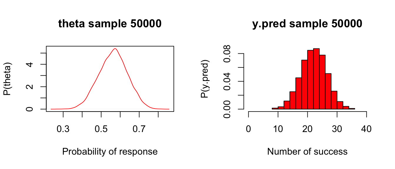
圖 97.2: Posterior and predictive distributions for Drug example
# # Or simply use the denplot() function from the mcmcplots package
# mcmcplots::denplot(post.jags, "theta")圖97.2左邊的圖,是前一次試驗結果的事後概率分布,20名患者中觀察到15名患者症狀改善。右邊的圖則是對下一次40人的試驗的結果做的預測,平均22.5名患者可能會有症狀改善,這個均值的標準差是4.3。
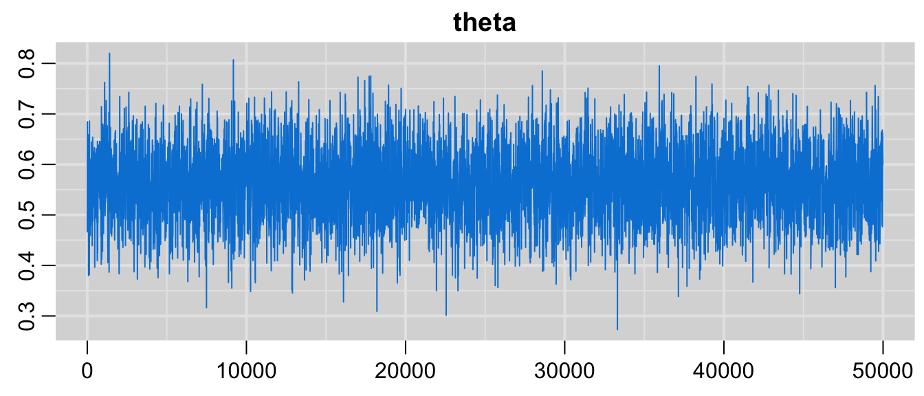
圖 97.3: Plot of the MCMC chain of the parameter, Drug example.
爲了比較,我們可以把精確計算獲得的答案和蒙特卡羅算法給出的預測做個比較:
- \(\theta:\)均值爲0.563,標準差是0.075;
- \(y_{\text{pred}}:\)均值22.51,標準差是4.31;
- 至少25名患者得到症狀改善的精確概率是 0.329。
97.3 正態分布(似然)數據的共軛先驗概率
例子:英國各地自來水公司依照法律規定,需要定期監測自己公司生產的自來水中三氯甲烷(trihalomethane, THM)的濃度。一年之中,每個公司都會在各個時期,不同的供水區域進行水樣的採集。假設現在我們需要來估計某個供水區域的自來水中三氯甲烷的濃度。
已知已經進行了兩次取樣,監測到三氯甲烷濃度分別是 \(y_1 = 128\mu g/l, y_2 = 132 \mu g/l\)。兩次監測的均值爲 \(130 \mu g/l\)。如果,這一片固定供水區域監測三氯甲烷濃度時檢測值的標準差是已知的 \(\sigma = 5\mu g/l\),那麼問題是,在這片固定供水區域的三氯甲烷濃度的估計值\((\theta)\)能否計算?
一個只有概率論知識的統計專家是這樣計算的:
- 樣本均值 \(\bar y = 130 \mu g/l\)是總體均值 \(\theta\) 的一次估計;
- 它的標準誤是 \(\frac{\sigma}{\sqrt{n}} = 5/\sqrt{2} = 3.5 \mu g/l\)。
- 然後這兩次測量的結果告訴我們總體均值的點估計和95%信賴區間是: \(\bar y \pm 1.96 \times \sigma/\sqrt{n} = 130 \pm 1.96\times3.5 = (123.1, 136.9) \mu g /l\)
但是一個擁有了貝葉斯統計學知識的統計專家則會是這樣思考的:
這個模型中,我們知道似然(likelihood)是一個正態分布:\(y_i \sim N(\theta, \sigma^2) (i = 1, \dots, n)\),且這裏的標準差是已知的 \(\sigma = 5\mu g/l\)。那麼我們給均值這個參數 \(\theta\) 一個怎樣的先驗概率分布呢?
\[ \theta \sim N(\mu, \omega^2) \]
- 先驗概率分布的方差 \(\omega^2\) 常可以用數據的方差來表達:\(\omega^2 = \sigma^2/n_0\)。
- 這裏的 \(n_0\),可以被解釋爲隱藏的先驗概率樣本量(implicit prior sample size)。
在 BUGS/JAGS 標記法中,正態分布的代碼是 y ~ dnorm(theta, tau),其中 tau 是方差的倒數(又叫做精確度)。
這時候我們需要一些過去同一家供水廠監測三氯甲烷時濃度的數據來給這個先驗概率分布一些提示。例如翻閱記錄我們發現來自同一家自來水公司,在其他供水區域的三氯甲烷濃度均值是 \(120 \mu g/l\),標準差是 \(10 \mu g/l\)。這就提供了 \(N(120, 10^2)\) 作爲 \(\theta\) 的先驗概率分布。這時我們把先驗概率分布的標準差用觀測區域的標準差來表達: \(\omega^2 = \sigma^2/n_0\),此時 \(n_0 = \sigma^2/\omega^2 = 5^2/10^2 = 0.25\)。那麼先驗概率分布可以被表達成 \(\theta \sim N(120, \sigma^2/0.25)\)。如果 \(n_0\) 靠近 \(0\),那麼根據這個方程我們知道先驗概率分布的方差就會變大,意味着先驗概率給出的信息越不精確,分布越”平坦(flatter)“。
此時貝葉斯統計專家把似然和先驗概率分布結合起來,計算事後概率分布:
\[ \begin{aligned} \theta | \mathbf{y} & \sim N(\frac{n_0 + n\bar y}{n_0 + n}, \frac{\sigma^2}{n_0 + n})\\ & \sim N(\frac{0.25\times 120 + 2 \times 130}{0.25 + 2}, \frac{5^2}{0.25 + 2}) \\ & = N(128.9, 3.33^2 ) \end{aligned} \]
貝葉斯算法給出的事後概率分布的95%可信區間則是 \((122.4, 135.4) \mu g/l\)。
事後概率分布的均值\(\frac{n_0 + n\bar y}{n_0 + n}\)其實是先驗概率均值,和觀測數據均值之間加權之後的綜合值,它們加的權重,分別是各自的精確度(相對樣本量 relative sample size)。這其實告訴我們,觀測數據和先驗概率二者結合之時,需要各自妥協。(a compromise between the likelihood and the prior)
事後概率分布的方差也是和先前提到的先驗概率樣本量有密切關系。它是觀測數據的方差除以觀測樣本量和先驗概率樣本量之和。
當然,當你的觀測數據樣本量趨向於無窮大時 \(n \rightarrow \infty\),事後概率分布本身就接近與觀測數據的似然 \(p(\theta | \mathbf{y}) \rightarrow N(\bar y, \sigma^2/n)\)。也就是說觀測數據的信息量佔絕對主導,先驗概率分布,不再能提供太多有價值的信息,可以忽略不計了。
# prior function
xseq<-seq(80,180,.01)
densities<-dnorm(xseq, 120,10)

# Plot
plot(xseq, densities, col="darkgreen",xlab="mean THM concentration, ug/l (theta)",
     ylab="Density", type="l",lwd=2, cex=2,
     # main="PDF of Prior, likelihood, and posterior for THM example.",
     cex.axis=0.9, cex.lab = 1, ylim = c(0,0.12))

# normal likelihood function (likelihood)

Likelihood <- dnorm(xseq, 130, 5)

# Plot
points(xseq, Likelihood, col="darkred", type="l",lwd=2, cex=2)


# Posterior function

posterior <-  dnorm(xseq, 128.9, 3.33)

# Plot

points(xseq, posterior, col="black", type="l",lwd=2, cex=2)

legend("topright", c("Prior", "Likelihood", "Posterior"), bty = "n", lwd = 2,
       lty = c(1,1,1), col = c("darkgreen", "darkred", "black"))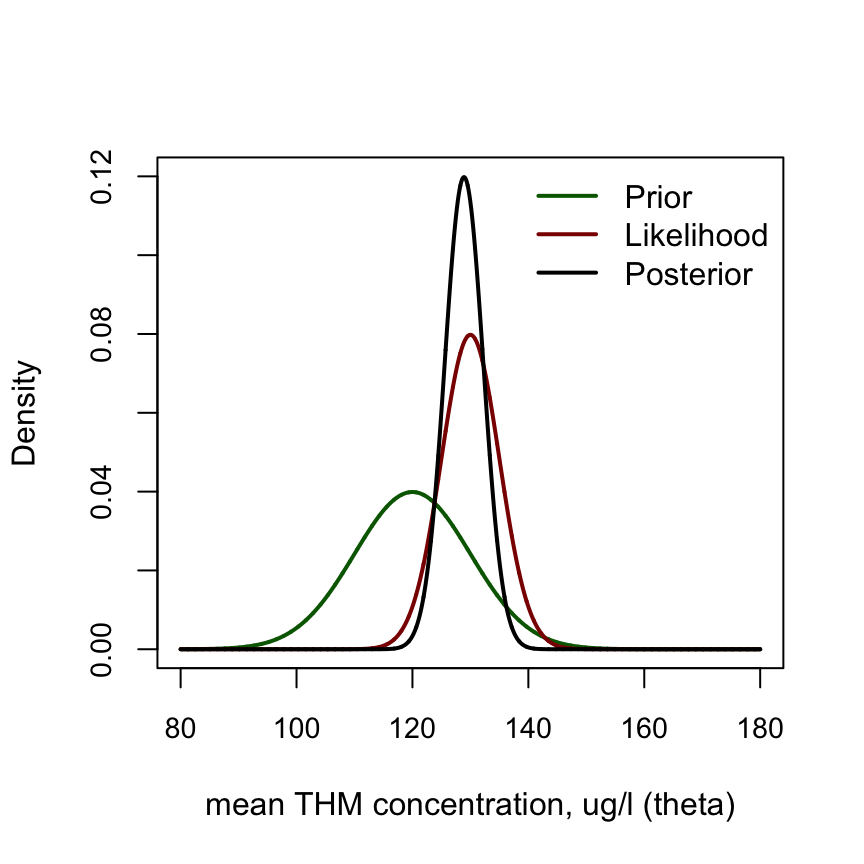
圖 97.4: PDF of Prior, likelihood and posterior for THM example.
97.4 泊淞分布(似然)數據的共軛先驗概率
接下來,我們把注意力轉到計數型數據的模型,泊淞分布上來。如果一組數據是計數型數據,\(y_1, y_2, \dots. , y_n\),它們可以被認爲是服從泊淞分布的話,它們的總體均值是\(\mu\),其似然(likelihood)方程可以寫作:
\[ p(\mathbf{y} | \mu) = \prod_i\frac{\mu^{y_i}e^{-\mu}}{y_i!} \]
那麼,經過前輩探索,我們知道,泊淞分布的似然它也有一個共軛先驗概率分布,是伽馬分布(Gamma distribution):
\[ p(\mu) = \text{Gamma}(a,b) = \frac{b^a}{\Gamma(a)}\mu^{a-1}e^{-b\mu} \]
伽馬分布是一個十分靈活的分布,適用於要求數據嚴格爲正的模型(positive quantities)。如果 \(\mu \sim \text{Gamma}(a,b)\):
\[ \begin{aligned} p(\mu | a,b) & = \frac{b^a}{\Gamma(a)}\mu^{a-1}e^{-b\mu}, \mu \in (0,\infty) \\ \text{E}(\mu |a,b) & = \frac{a}{b} \\ \text{V}(\mu |a,b) & = \frac{a}{b^2} \end{aligned} \]
它的模型在BUGS語言可以用 mu ~ dgamma(a,b) 來表述。伽馬分布還有如下的一些有趣的特徵:
- \(\text{Gamma}(1,b)\) 是均值爲 \(\frac{1}{b}\) 的指數分布。
- \(\text{Gamma}(\frac{v}{2},\frac{1}{2})\),其實是自由度爲 \(v\) 的卡方分布 \(\chi_v^2\)。
- \(\mu \sim \text{Gamma}(0,0)\) 其實等價於 \(p(\mu) \propto \frac{1}{\mu}\),或者 \(\log \mu \sim \text{Uniform}\)。
- 伽馬分布同時也是正態分布數據(似然)的精確度(方差的倒數,inverse variance or precision)共軛先驗概率。
- 伽馬分布也可以用於正向非對稱性分布(skewed positive valued quantities)的樣本分布。
下圖展示了一些常見伽馬分布的形狀:
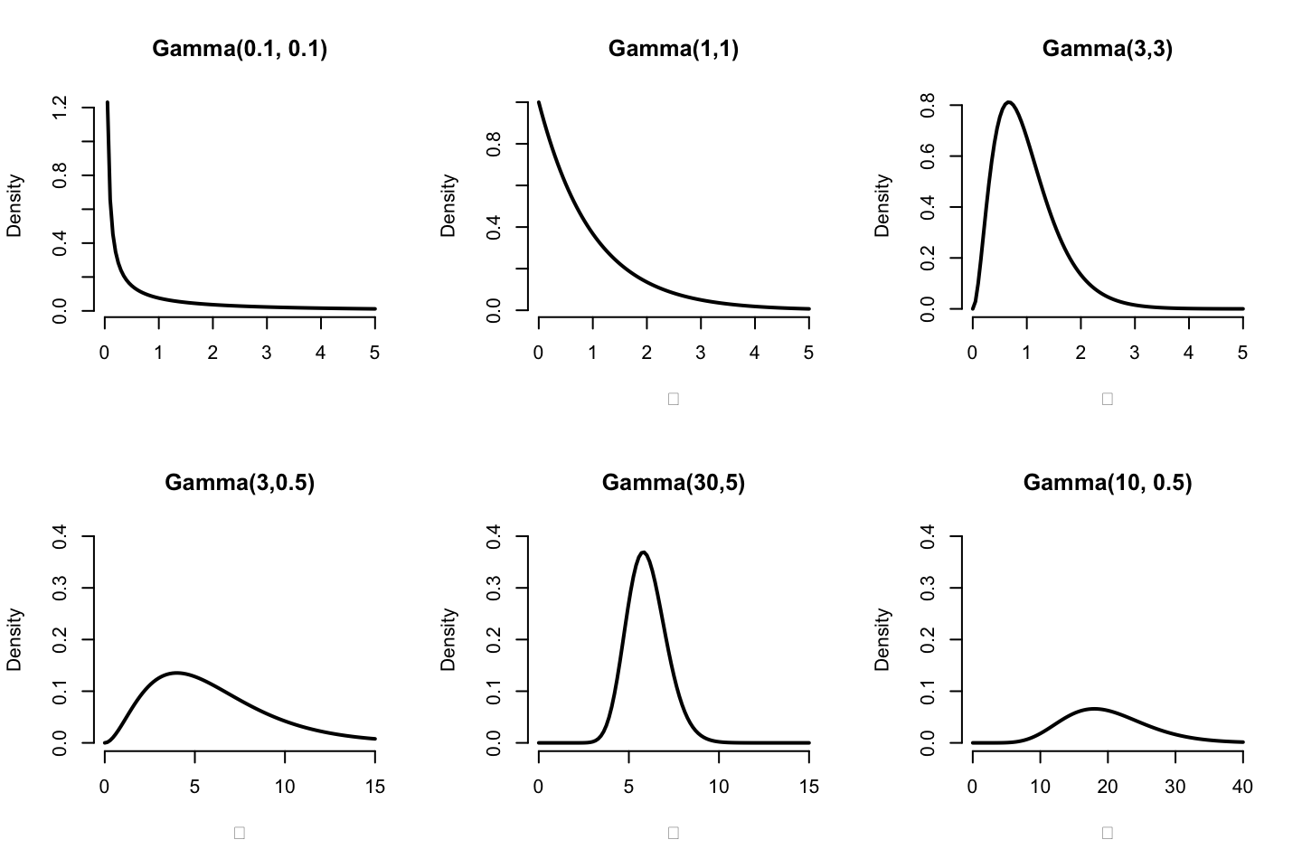
圖 97.5: Shape of some Gamma distribution functions for various values of a, b
將伽馬分布的概率方程和泊淞分布似然方程相結合,貝葉斯定理告訴我們,它會變成另外一個更新過後的伽馬分布:
\[ \begin{aligned} p(\mu | \mathbf{y}) & \propto p(\mu) p(\mathbf{y} | \mu) \\ & = \frac{b^a}{\Gamma(a)}\mu^{a-1}e^{-b\mu} \prod_{i=1}^ne^{-\mu}\frac{\mu^{y_i}}{y_i!} \\ & \propto \mu^{a + n\bar y -1} e^{-(b+n)\mu} \\ & = \text{Gamma}(a + n\bar y, b+n) \end{aligned} \]
這個新的伽馬分布的期望值是:
\[ E(\mu | \mathbf{y}) = \frac{a + n\bar y}{b + n} = \bar y (\frac{n}{n + b}) + \frac{a}{b}(1 - \frac{n}{n + b}) \]
也就是說事後概率分布的伽馬分布,它的均值(期望)是先驗概率分布的均值 \(\frac{a}{b}\) 和數據樣本均值 \(\bar y\) 相互妥協的結果。泊淞-伽馬分布的模型常常可以用於估計發病率(rate),或者相對危險度(relative risk),反而較少用於估計率數據的均值(mean of possion data)。
97.5 共軛先驗概率分布的總結
從這些共軛概率分布的結果和他們的特徵值的推導來看,我們發現:
- 事後概率分布的均值,總是將先驗概率分布均值和觀察數據的樣本均值相結合並且互相妥協之後的結果。
- 事後概率分布的標準差(方差),總是小於先驗概率分布的方差和觀察數據的樣本標準差的任何一個。
而且,當樣本數據的樣本量很大, \(n \rightarrow \infty\):
- 事後概率分布的均值都會無限接近觀察數據的樣本均值。\(\text{The posterior mean } \rightarrow \text{ the sample mean}\);
- 事後概率分布的標準差會無限接近觀察數據的樣本標準誤。\(\text{The posterior standard deviation } \rightarrow \text{ the standard error}\);
- 事後概率分布就不再依賴先驗概率分布了。
當事後概率分布,和先驗概率分布恰好都來自相同分布家族時,我們稱這樣的分布具有共軛性質(conjugacy)。此時,先驗概率分布的參數常常可以被解讀成爲先驗概率樣本(prior sample)。
這樣的分布我們總結一下常見的例子:
| Likelihood | Parameter | Prior | Posterior |
|---|---|---|---|
| Normal | mean | Normal | Normal |
| Normal | precision | Gamma | Gamma |
| Binomial | success prob. | Beta | Beta |
| Poisson | rate or mean | Gamma | Gamma |
共軛先驗概率分布在數學上是十分便利的,但是並不是所有的似然都能找到它的共軛概率分布做先驗概率。這時候我們就需要求助於計算機模擬試驗的威力,下一章我們會接觸到怎樣使用 Markov Chain Monte Carlo (MCMC)來克服我們找不到共軛先驗概率的似然時,後驗概率分布的計算。它的中文名被翻譯成馬爾可夫鏈蒙特卡羅。
97.6 Practical Bayesian Statistics 03
A. 新藥試驗模型
新藥臨牀試驗的BUGS模型可以寫作:
# Drug example - model code

model{
   theta    ~ dbeta(a,b)               # prior distribution
   y        ~ dbin(theta,n)            # sampling distribution
   y.pred   ~ dbin(theta,m)            # predictive distribution
   P.crit   <- step(y.pred-ncrit+0.5)  # =1 if y.pred >= ncrit, 0 otherwise
}
這個模型中 theta 是藥物的陽性反應率(有效率, response rate);y.pred是40名未來患者中可能出現陽性反應的人數(number of positive response in 40 future patients)。P.crit 是用來表示患者中有25名或者更多的人有陽性反應時的指示變量(indicator variable)。
新藥試驗的數據則可以寫爲:
# Drug example - data
# values for a, b, m, n, ncrit could alternatively have been given in model description

list(
a = 9.2,    # parameters of prior distribution
b = 13.8,
y = 15,     # number of successes
n = 20,     # number of trials
m = 40,     # future number of trials
ncrit = 25) # critical value of future successes
把這裏的模型保存稱爲 drug-model.txt文件,把數據保存成 drug-data.txt文件,我們來試着用OpenBUGS/JAGS跑這個模型:
# Codes for OpenBUGS

# # Step 1 check model
# modelCheck(paste(bugpath, "/backupfiles/drug-model.txt", sep = ""))
# # Load the data
# modelData(paste(bugpath, "/backupfiles/drug-data.txt", sep = ""))
# # compile the model
# modelCompile(numChains = 1)
# # There is no need to provide initial values as
# # they are aleady provided in the model specification
# modelGenInits() #
# # Set monitors on nodes of interest#### SPECIFY, WHICH PARAMETERS TO TRACE:
# parameters <- c("P.crit", "theta", "y.pred")
# samplesSet(parameters)

# # Generate 10000 iterations
# modelUpdate(10000)
# #### SHOW POSTERIOR STATISTICS
# sample.statistics <- samplesStats("*")
# print(sample.statistics)

# Codes for R2JAGS


Dat <- list(a = 9.2,             # parameters of prior distribution
            b = 13.8,
            y = 15,              # number of successes in completed trial
            n = 20,              # number of patients in completed trial
            m = 40,              # number of patients in future trial
            ncrit = 25)          # critical value of future successes

# fit use R2jags package

post.jags <- jags(
  data = Dat,
  parameters.to.save = c("P.crit", "theta", "y.pred"),
  n.iter = 10100,
  model.file = paste(bugpath,
                     "/backupfiles/drug-model.txt",
                     sep = ""),
  n.chains = 1,
  n.thin = 1,
  n.burnin = 100,
  progress.bar = "none")
## Compiling model graph
## Resolving undeclared variables
## Allocating nodes
## Graph information:
## Observed stochastic nodes: 1
## Unobserved stochastic nodes: 2
## Total graph size: 12
##
## Initializing model## Inference for Bugs model at "/Users/chaoimacmini/Downloads/LSHTMlearningnote/backupfiles/drug-model.txt", fit using jags,
## 1 chains, each with 10100 iterations (first 100 discarded)
## n.sims = 10000 iterations saved
## mu.vect sd.vect 2.5% 25% 50% 75% 97.5%
## P.crit 0.334 0.472 0.000 0.000 0.000 1.000 1.000
## theta 0.563 0.074 0.416 0.513 0.564 0.613 0.708
## y.pred 22.523 4.304 14.000 20.000 23.000 26.000 31.000
## deviance 6.637 2.378 3.382 4.873 6.199 7.916 12.404
##
## DIC info (using the rule, pD = var(deviance)/2)
## pD = 2.8 and DIC = 9.5
## DIC is an estimate of expected predictive error (lower deviance is better).此時我們獲得我們關心的各個事後概率分佈描述,其中陽性反應率的點估計是0.563,其95%可信區間是(0.412, 0.707)。40名患者中25人或者以上出現有療效反應的概率是32.4%。
請繪製theta的事後概率分佈的密度曲線,以及y.pred的預測概率分佈:
#### PLOT THE DENSITY and HISTOGRAMS OF THE SAMPLED VALUES
par(mfrow=c(1,2))
Theta <- ggSample %>%
  filter(Parameter == "theta")
Y <- ggSample %>%
  filter(Parameter == "y.pred")
plot(density(Theta$value), main = "theta sample 10000",
     ylab = "P(theta)", xlab = "Probability of response", col = "red")
hist(Y$value, main = "y.pred sample 10000", ylab = "P(y.pred)",
     xlab = "Number of success", col = "red", prob = TRUE,xlim = c(0, 40))
圖 97.6: Posterior and predictive distributions for Drug example
比較一下這裏的模型和我們前一章的練習中的模型,
- Model from Practical 2
#  Monte Carlo predictions for Drug example

model{
    theta   ~ dbeta(9.2,13.8)          # prior distribution
    y         ~ dbin(theta,20)         # sampling distribution
    P.crit   <- step(y-14.5)           # =1 if y >= 15, 0 otherwise
}- Model from Practical 3
# Drug example - model code

model{
   theta    ~ dbeta(a,b)               # prior distribution
   y        ~ dbin(theta,n)            # sampling distribution
   y.pred   ~ dbin(theta,m)            # predictive distribution
   P.crit   <- step(y.pred-ncrit+0.5)  # =1 if y.pred >= ncrit, 0 otherwise
# data
y <- 15
}
這兩個模型的構成基本上是相同的,最重要的不同點在於,Practical 2中的 MC分析中沒有關於該次試驗的觀測數據 y,也就是20名患者中陽性反應,療效顯著的患者人數。所以,該模型不能從試驗數據中”學習”,導致 OpenBUGS/JAGS 其實在進行 MC 模擬試驗時僅僅是從先驗概率分佈 \(\text{Beta}(9.2, 13.8)\) 中隨機採樣對結果做出預測。在 Practical 3的模型裏,我們把試驗數據加入到了模型裏面 y <- 15,所以OpenBUGS/JAGS此時識別了本次試驗數據是20人中15人有效,接下來它就知道需要做事後概率分佈的計算而不是一個結果的預測。獲得事後概率分佈之後,OpenBUGS/JAGS也就開始從事後概率分佈當中獲取隨機樣本。然後我們需要在模型中加入新的變量來預測下一次如果做40人的研究時,可能出現的事後概率分佈。
如果把模型中陽性反應率theta的先驗概率分佈改成一個沒有太多信息的,連續型均勻分佈(uniform distribution),例如 \(\text{Uniform}(0,1)\),或者是 \(\text{Beta}(1,1)\)。MC結果會變成怎樣呢?
先驗概率爲連續型均勻分佈的BUGS模型和數據可以寫成是:
# Drug example - model code

model{
   theta    ~ dunif(0,1)               # prior distribution uniform distribution
   y        ~ dbin(theta,n)            # sampling distribution for n observed patients
   y.pred   ~ dbin(theta,m)            # predictive distribution for m new patients
   P.crit   <- step(y.pred-ncrit+0.5)  # =1 if y.pred >= ncrit, 0 otherwise
}
list(
y = 15, # number of successes
n = 20, # number of trials
m = 40, # future number of trials
ncrit = 25 # critical value of future successes
)# Codes for OpenBUGS
# # Step 1 check model
# modelCheck(paste(bugpath, "/backupfiles/drug-modeluniform.txt", sep = ""))
# # Load the data
# modelData(paste(bugpath, "/backupfiles/drug-datauniform.txt", sep = ""))
# # compile the model
# modelCompile(numChains = 1)
# # There is no need to provide initial values as
# # they are aleady provided in the model specification
# modelGenInits() #
# # Set monitors on nodes of interest#### SPECIFY, WHICH PARAMETERS TO TRACE:
# parameters <- c("P.crit", "theta", "y.pred")
# samplesSet(parameters)
#
# # Generate 10000 iterations
# modelUpdate(10000)
# #### SHOW POSTERIOR STATISTICS
# sample.statistics <- samplesStats("*")
# print(sample.statistics)
# Codes for R2JAGS
Dat <- list(
y = 15, # number of successes
n = 20, # number of trials
m = 40, # future number of trials
ncrit = 25 # critical value of future successes
)
# fit use R2jags package
post.jags <- jags(
data = Dat,
parameters.to.save = c("P.crit", "theta", "y.pred"),
n.iter = 10100,
model.file = paste(bugpath,
"/backupfiles/drug-modeluniform.txt",
sep = ""),
n.chains = 1,
n.thin = 1,
n.burnin = 100,
progress.bar = "none")## Compiling model graph
## Resolving undeclared variables
## Allocating nodes
## Graph information:
## Observed stochastic nodes: 1
## Unobserved stochastic nodes: 2
## Total graph size: 12
##
## Initializing model## Inference for Bugs model at "/Users/chaoimacmini/Downloads/LSHTMlearningnote/backupfiles/drug-modeluniform.txt", fit using jags,
## 1 chains, each with 10100 iterations (first 100 discarded)
## n.sims = 10000 iterations saved
## mu.vect sd.vect 2.5% 25% 50% 75% 97.5%
## P.crit 0.835 0.371 0.000 1.000 1.000 1.000 1.000
## theta 0.728 0.093 0.530 0.668 0.735 0.795 0.889
## y.pred 29.101 4.665 19.000 26.000 29.000 33.000 37.000
## deviance 4.141 1.331 3.197 3.286 3.628 4.443 7.944
##
## DIC info (using the rule, pD = var(deviance)/2)
## pD = 0.9 and DIC = 5.0
## DIC is an estimate of expected predictive error (lower deviance is better).這個結果則提示,如果使用連續型均勻分佈的先驗概率,新藥試驗的陽性反應率是0.73,95%可信區間是(0.53, 0.89)。根據這個試驗結果對下次40人的試驗做預測時,認爲40人中大於或者等於25人有顯著療效(陽性反應)的概率會有0.84。
B. THM 三氯甲烷濃度實例
在飲用水檢測三氯甲烷濃度這個試驗中,我們已知濃度的方差,希望通過貝葉斯方法推斷其均值。
以下是我們需要思考的問題:
- 在這個供水區域內,三氯甲烷的濃度均值是多少?
- 兩次測量濃度的數據,它的似然是怎樣的? 如果可以假定三氯甲烷濃度服從正態分佈,那麼似然就是正態分佈似然:
y[i] ~ N(theta, sigma^2)。 - 在上面提到的正態分佈似然中,有哪些參數,哪個是已知的哪個是未知的?
theta區域濃度的均值未知,sigma區域濃度的方差是給定的(已知的)。 - 哪個參數需要在模型中給出先驗概率分佈?該怎樣指定這個先驗概率分佈才合理?
theta,區域濃度均值需要給它指定一個先驗概率分佈,正態分佈數據均值的先驗概率分佈可以使用正態分佈。
# THM model:
model {
   # data
   # y[1] <- 128
   # y[2] <- 132
   # tau <- 1/pow(5, 2)

   for(i in 1:2) {
      y[i] ~ dnorm(theta, tau)
   }

   # informative prior
   theta ~ dnorm(120, prec)
   prec <- 1/100

   # vague prior
   # theta ~ dnorm(0, 0.000001)
   # OR
   # theta ~ dunif(-10000, 10000)
}
在BUGS語言中,正態分佈用 dnorm(theta, tau),其中 theta 爲均值,tau 是精確度(precision = 1/variance),它是方差的倒數。
# Codes for R2JAGS


Dat <- list(
y = c(128, 132),                       # observed
tau = 1/(5^2)
)

# fit use R2jags package

post.jags <- jags(
  data = Dat,
  parameters.to.save = c("theta"),
  n.iter = 10100,
  model.file = paste(bugpath,
                     "/backupfiles/thm-model.txt",
                     sep = ""),
  n.chains = 1,
  n.thin = 1,
  n.burnin = 100,
  progress.bar = "none")
## Compiling model graph
## Resolving undeclared variables
## Allocating nodes
## Graph information:
## Observed stochastic nodes: 2
## Unobserved stochastic nodes: 1
## Total graph size: 8
##
## Initializing model## Inference for Bugs model at "/Users/chaoimacmini/Downloads/LSHTMlearningnote/backupfiles/thm-model.txt", fit using jags,
## 1 chains, each with 10100 iterations (first 100 discarded)
## n.sims = 10000 iterations saved
## mu.vect sd.vect 2.5% 25% 50% 75% 97.5%
## theta 128.868 3.342 122.241 126.547 128.867 131.137 135.377
## deviance 11.429 1.402 10.434 10.537 10.899 11.750 15.521
##
## DIC info (using the rule, pD = var(deviance)/2)
## pD = 1.0 and DIC = 12.4
## DIC is an estimate of expected predictive error (lower deviance is better).# OpenBUGS code:
# # Step 1 check model
# modelCheck(paste(bugpath, "/backupfiles/thm-model.txt", sep = ""))
#
# # compile the model
# modelCompile(numChains = 1)
# # There is no need to provide initial values as
# # they are aleady provided in the model specification
# modelGenInits() #
# # Set monitors on nodes of interest#### SPECIFY, WHICH PARAMETERS TO TRACE:
# parameters <- c("theta")
# samplesSet(parameters)
# # Generate 10000 iterations
# modelUpdate(10000)
# #### SHOW POSTERIOR STATISTICS
# sample.statistics <- samplesStats("*")
# print(sample.statistics)所以這個區域三氯甲烷的事後均值和95%可信區間分別是 128.9 (122.3, 135.4)。和我們之前用精確計算法給出的結果相同/相近。
如果在這個模型中,我們嘗試沒有信息的先驗概率分佈,結果會怎樣呢?
# Codes for R2JAGS


Dat <- list(
y = c(128, 132),                       # observed
tau = 1/(5^2)
)

# fit use R2jags package

post.jags <- jags(
  data = Dat,
  parameters.to.save = c("theta"),
  n.iter = 10100,
  model.file = paste(bugpath,
                     "/backupfiles/THM-vaguemodel.txt",
                     sep = ""),
  n.chains = 1,
  n.thin = 1,
  n.burnin = 100,
  progress.bar = "none")
## Compiling model graph
## Resolving undeclared variables
## Allocating nodes
## Graph information:
## Observed stochastic nodes: 2
## Unobserved stochastic nodes: 1
## Total graph size: 6
##
## Initializing model## Inference for Bugs model at "/Users/chaoimacmini/Downloads/LSHTMlearningnote/backupfiles/THM-vaguemodel.txt", fit using jags,
## 1 chains, each with 10100 iterations (first 100 discarded)
## n.sims = 10000 iterations saved
## mu.vect sd.vect 2.5% 25% 50% 75% 97.5%
## theta 130.002 3.508 123.113 127.673 129.999 132.324 137.036
## deviance 11.418 1.414 10.434 10.530 10.866 11.729 15.391
##
## DIC info (using the rule, pD = var(deviance)/2)
## pD = 1.0 and DIC = 12.4
## DIC is an estimate of expected predictive error (lower deviance is better).# OpenBUGS code:
# # Step 1 check model
# modelCheck(paste(bugpath, "/backupfiles/THM-vaguemodel.txt", sep = ""))
#
# # compile the model
# modelCompile(numChains = 1)
# # There is no need to provide initial values as
# # they are aleady provided in the model specification
# modelGenInits() #
# # Set monitors on nodes of interest#### SPECIFY, WHICH PARAMETERS TO TRACE:
# parameters <- c("theta")
# samplesSet(parameters)
#
# # Generate 10000 iterations
# modelUpdate(10000)
# #### SHOW POSTERIOR STATISTICS
# sample.statistics <- samplesStats("*")
# print(sample.statistics)MC試驗10000次給出的事後均值是129.9,它和樣本均值相同,因爲此時我們給模型一個幾乎不含有效信息的先驗概率分佈時,意味着我們讓試驗獲得的數據做完全主導作用,“data speak for themselves”。
C. Disease risk in a small area
下面的BUGS/JAGS模型代碼可以用來進行泊淞-伽馬分布似然的MC計算。在這個例子中,在某個區域我們觀察到5例白血病新病例,已知該區域的年齡性別標準化發病期望病例數是\(E = 2.8\)。注意看我們在代碼中加入了兩種不同類型的先驗概率分布,一個是沒有太多信息的(vague prior distribution)dgamma(0.1, 0.1),一個則是有一定信息的(informative prior, stribution) dgamma(48, 40)。我們把兩個先驗概率分布同時加在一個模型裏,這是十分便於進行兩種先驗概率對結果的影響的比較的手段。你當然可以把它寫成兩個不同的模型。注意模型代碼是如何表示事後概率分布和計算相對危險度比(relative risk)大於1的概率的。
model {

    lambda[1]  ~ dgamma(0.1, 0.1)   # vague prior distribution
    lambda[2]  ~ dgamma(48, 40)     # informative prior distribution

    y[1]  ~ dpois(mu[1])             # sampling distribution
    mu[1] <- lambda[1] * 2.8

    # repeat for second model
    y[2] ~ dpois(mu[2])             # sampling distribution
    mu[2] <- lambda[2] * 2.8

  # Is relative risk > 1
  P.excess[1] <- step(lambda[1] - 1)
  P.excess[2] <- step(lambda[2] - 1)

    # data
    # y[1] <- 5
    # y[2] <- 5             # replicate data to fit both models together

}
# Codes for R2JAGS
Dat <- list(
y = c(5, 5) # replicate data to fit both models together
)
# fit use R2jags package
post.jags <- jags(
data = Dat,
parameters.to.save = c("P.excess[1]", "P.excess[2]", "lambda[1]", "lambda[2]"),
n.iter = 10100,
model.file = paste(bugpath,
"/backupfiles/disease-model.txt",
sep = ""),
n.chains = 1,
n.thin = 1,
n.burnin = 100,
progress.bar = "none")## Compiling model graph
## Resolving undeclared variables
## Allocating nodes
## Graph information:
## Observed stochastic nodes: 2
## Unobserved stochastic nodes: 2
## Total graph size: 15
##
## Initializing model## Inference for Bugs model at "/Users/chaoimacmini/Downloads/LSHTMlearningnote/backupfiles/disease-model.txt", fit using jags,
## 1 chains, each with 10100 iterations (first 100 discarded)
## n.sims = 10000 iterations saved
## mu.vect sd.vect 2.5% 25% 50% 75% 97.5%
## P.excess[1] 0.848 0.359 0.000 1.000 1.000 1.000 1.000
## P.excess[2] 0.928 0.259 0.000 1.000 1.000 1.000 1.000
## lambda[1] 1.773 0.783 0.590 1.202 1.652 2.225 3.590
## lambda[2] 1.239 0.169 0.933 1.122 1.231 1.349 1.590
## deviance 8.650 1.482 7.170 7.708 8.215 9.071 12.721
##
## DIC info (using the rule, pD = var(deviance)/2)
## pD = 1.1 and DIC = 9.7
## DIC is an estimate of expected predictive error (lower deviance is better).# # Step 1 check model
# modelCheck(paste(bugpath, "/backupfiles/disease-model.txt", sep = ""))
#
# # compile the model
# modelCompile(numChains = 1)
# # There is no need to provide initial values as
# # they are aleady provided in the model specification
# modelGenInits() #
# # Set monitors on nodes of interest#### SPECIFY, WHICH PARAMETERS TO TRACE:
# parameters <- c("P.excess[1]", "P.excess[2]", "lambda[1]", "lambda[2]")
# samplesSet(parameters)
#
# # Generate 10000 iterations
# modelUpdate(10000)
# #### SHOW POSTERIOR STATISTICS
# sample.statistics <- samplesStats("*")
# print(sample.statistics)在沒有信息的先驗概率(dgamma(0.1, 0.1))分布條件下,該地區可能有較高白血病發病率的概率是85%,但是在有參考價值信息的先驗概率分布(dgamma(48, 40))條件下,該地區可能有較高白血病發病率的概率是93%。所以,盡管相對危險度(relative risk)的事後均值在沒有信息的先驗概率分布條件下比較高(lambda[1] = 1.770 > lambda[2] = 1.238),但是沒有信息的先驗概率分布條件下,這個相對危險度大於1的概率(85%)要比有信息的先驗概率分布條件下相對危險度大於1的概率要低(93%)。這是因爲在沒有信息的先驗概率分布條件下,相對危險度估計本身有太多的不確定性(uncertainty,圖97.7)。
#
# # Step 1 check model
# modelCheck(paste(bugpath, "/backupfiles/disease-model.txt", sep = ""))
#
# # compile the model
# modelCompile(numChains = 1)
# # There is no need to provide initial values as
# # they are aleady provided in the model specification
# modelGenInits() #
# # Set monitors on nodes of interest#### SPECIFY, WHICH PARAMETERS TO TRACE:
# parameters <- c("P.excess[1]", "P.excess[2]", "lambda[1]", "lambda[2]")
# samplesSet(parameters)
#
# # Generate 10000 iterations
# modelUpdate(10000)


#### PUT THE SAMPLED VALUES IN ONE R DATA FRAME:
# chain <- data.frame(P.excess1 = samplesSample("P.excess[1]"),
#                     P.excess2 = samplesSample("P.excess[2]"),
#                     lambda1 = samplesSample("lambda[1]"),
#                     lambda2 = samplesSample("lambda[2]"))
Simulated <- coda::as.mcmc(post.jags)
#### PUT THE SAMPLED VALUES IN ONE R DATA FRAME:
ggSample <- ggmcmc::ggs(Simulated)

Lambda1 <- ggSample %>%
  filter(Parameter == "lambda[1]")
Lambda2 <- ggSample %>%
  filter(Parameter == "lambda[2]")

boxplot(Lambda1$value,Lambda2$value, col = "green", ylab = "lambda",
        outline=FALSE, main = "boxplot: lambda", ylim = c(0,4),
        names = c("1", "2"))
abline(h = 1.5)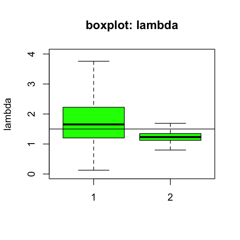
圖 97.7: Box plots of relative risk (lambda) of leukaemia under different priors (vague = 1, informative = 2).
圖 97.7的箱式圖也告訴我們,相對危險度的事後概率分布在有信息的先驗概率分布條件下要精確得多,其標準差sd[2] = 0.17也要小得多 sd[1] = 0.78。所以,此時,先驗概率分布對我們的事後概率分布推斷產生了較大的影響,有信息的先驗概率分布把相對危險度的估計值更加拉近了1的同時(more realistic),也使得相對危險度的事後概率估計變得更加精確。
接下來,假設我們在該區域進行了更長時間的觀察,收集到100個新的白血病病例,同時在這段時間內病例的期望值只有56例。據此,重新改寫這個模型,在兩種先驗概率分布條件下,此時由於觀察數據信息量的增加,相對危險度的事後估計有怎樣的變化?
model {

    lambda[1]  ~ dgamma(0.1, 0.1)   # vague prior distribution
    lambda[2]  ~ dgamma(48, 40)     # informative prior distribution

    y[1]  ~ dpois(mu[1])             # sampling distribution
    mu[1] <- lambda[1] * 56          # the expectation changed from 2.8 to 56

    # repeat for second model
    y[2] ~ dpois(mu[2])             # sampling distribution
    mu[2] <- lambda[2] * 56         # the expectation changed from 2.8 to 56

  # Is relative risk > 1
  P.excess[1] <- step(lambda[1] - 1)
  P.excess[2] <- step(lambda[2] - 1)

    # data
    # y[1] <- 100             # the observed new cases changed from 5 to 100
    # y[2] <- 100             # replicate data to fit both models together

}
# Codes for R2JAGS
Dat <- list(
y = c(100, 100) # the observed new cases changed from 5 to 100
)
# fit use R2jags package
post.jags <- jags(
data = Dat,
parameters.to.save = c("P.excess[1]", "P.excess[2]", "lambda[1]", "lambda[2]"),
n.iter = 10100,
model.file = paste(bugpath,
"/backupfiles/disease-modelupdated.txt",
sep = ""),
n.chains = 1,
n.thin = 1,
n.burnin = 100,
progress.bar = "none")## Compiling model graph
## Resolving undeclared variables
## Allocating nodes
## Graph information:
## Observed stochastic nodes: 2
## Unobserved stochastic nodes: 2
## Total graph size: 15
##
## Initializing model## Inference for Bugs model at "/Users/chaoimacmini/Downloads/LSHTMlearningnote/backupfiles/disease-modelupdated.txt", fit using jags,
## 1 chains, each with 10100 iterations (first 100 discarded)
## n.sims = 10000 iterations saved
## mu.vect sd.vect 2.5% 25% 50% 75% 97.5%
## P.excess[1] 1.000 0.000 1.000 1.000 1.000 1.000 1.000
## P.excess[2] 1.000 0.000 1.000 1.000 1.000 1.000 1.000
## lambda[1] 1.785 0.180 1.452 1.660 1.778 1.905 2.153
## lambda[2] 1.544 0.128 1.304 1.457 1.540 1.628 1.804
## deviance 16.606 2.821 13.110 14.480 16.027 18.002 23.628
##
## DIC info (using the rule, pD = var(deviance)/2)
## pD = 4.0 and DIC = 20.6
## DIC is an estimate of expected predictive error (lower deviance is better).# OpenBUGS codes:
# # Step 1 check model
# modelCheck(paste(bugpath, "/backupfiles/disease-modelupdated.txt", sep = ""))
#
# # compile the model
# modelCompile(numChains = 1)
# # There is no need to provide initial values as
# # they are aleady provided in the model specification
# modelGenInits() #
# # Set monitors on nodes of interest#### SPECIFY, WHICH PARAMETERS TO TRACE:
# parameters <- c("P.excess[1]", "P.excess[2]", "lambda[1]", "lambda[2]")
# samplesSet(parameters)
#
# # Generate 10000 iterations
# modelUpdate(10000)
# #### SHOW POSTERIOR STATISTICS
# sample.statistics <- samplesStats("*")
# print(sample.statistics)有了更多的觀察數據的模型,我們看到,相對危險度的事後估計lambda[1], lambda[2]都變得更加精確了,有了更小的標準差。這和我們的預期相同,因爲觀察數據增加自然會提高相對危險度估計的精確度。可是,我們發現在沒有信息的先驗概率分布條件下,相對危險度的事後估計幾乎沒有太大的變化(1.783 v.s. 1.770)。相反地,有信息的先驗概率分布條件下,相對危險度的事後估計比之前增加了不少(1.540 v.s. 1.238)。這主要是因爲,現在我們得到更多的觀察數據,這些數據得到的信息被給予了更多的權重,且觀察數據提示相對危險度應該要比較大(100/56 = 1.786)。
盡管觀察數據確實給模型提供了較多的有價值的信息,你會發現,我們使用的第二個先驗概率分布(也就是有信息的先驗概率分布)仍然對相對危險度的事後估計起到了相當的影響(the prior variance is 0.03, giving prior sd of 0.17)。這也是因爲這個先驗概率分布給出的信息量,幾乎相當於觀察數據給出的信息量(二者的標準差很接近)。另外一種理解此現象的方法是看事後概率分布推導出的新的伽馬分布的計算式:
\[ \begin{aligned} p(\lambda | y, E) & \propto p(\lambda) p (y | \lambda, E) \\ & \propto \frac{b^a}{\Gamma(a)}\lambda^{a-1}e^{-b\lambda} \frac{(\lambda E)^ye^{-\lambda E}}{y!} \\ & \propto \lambda^{a + y -1}e^{-(b+E)\lambda} \\ & = \text{Gamma}(a + y, b + E) \end{aligned} \]
由於事後伽馬分布的方差(標準差)主要由第二個參數\((b + E)\)決定,從上面的公式推導我們可以看見,事後伽馬分布的第二個參數\((b + E)\),分別是先驗概率分布的第二個參數\((b = 40)\),和觀察數據的期望值\((E = 56)\)。由於這兩個數值大小接近,所以我們也可以理解此時先驗概率提供的信息和我們觀察數據提供的信息旗鼓相當。另外,在這個新的觀察數據條件下,我們無論使用哪個先驗概率分布做條件,都獲得了100%的結果也就是這個特定區域的白血病發病率大於期望值的概率是100%。也就是我們此時有100%的把握認爲這個特定區域的白血病發病率較高。
#### PUT THE SAMPLED VALUES IN ONE R DATA FRAME:
# chain <- data.frame(P.excess1 = samplesSample("P.excess[1]"),
#                     P.excess2 = samplesSample("P.excess[2]"),
#                     lambda1 = samplesSample("lambda[1]"),
#                     lambda2 = samplesSample("lambda[2]"))
Simulated <- coda::as.mcmc(post.jags)
#### PUT THE SAMPLED VALUES IN ONE R DATA FRAME:
ggSample <- ggmcmc::ggs(Simulated)

Lambda1 <- ggSample %>%
  filter(Parameter == "lambda[1]")
Lambda2 <- ggSample %>%
  filter(Parameter == "lambda[2]")

boxplot(Lambda1$value,Lambda2$value, col = "green", ylab = "lambda",
        outline=FALSE, main = "boxplot: lambda", ylim = c(0,4),
        names = c("1", "2"))
abline(h = 1.66)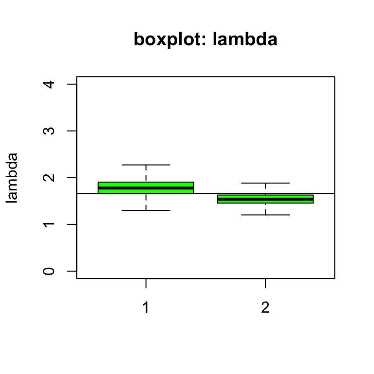
圖 97.8: Box plots of relative risk (lambda) of leukaemia under different priors (vague = 1, informative = 2) with more observations.
D. James Bond Example.
007邦德喝了16杯馬丁尼酒,每飲一杯,都被問道那杯馬丁尼酒是被調酒師用搖的(shaken)還是用攪拌的(stired)調制的。結果在這邦德喝過的16杯馬丁尼酒中,他居然答對了13杯。(007就是流弊)
嘗試修改新藥試驗的模型代碼,用均一分布作爲參數\(\theta\)的先驗概率分布,你是否能進行一個貝葉斯分析來回答這個問題:“邦德能夠正確區分一杯馬丁尼酒的調制方法的概率是多少?”
那如果把這個問題稍微改變一下,“邦德能夠區分馬丁尼酒的調制方法的概率是多少?(what is the probability that James Bond has at least some ability to tell the difference between shaken and stirred martinis?i.e. better than guessing)”你能回答嗎?
假定這樣一個場景,你和另外三個朋友在酒吧遇見了邦德,你們每個人都說要和邦德玩品酒的遊戲,如果邦德能準確分辨出馬丁尼酒的調制方法,你們就付那一杯酒錢,如果邦德答錯了,那他要把酒錢付給你們。在這樣的場景下,已知邦德能分辨16杯馬丁尼酒中的13杯,你們4人有多大的概率能把酒錢都賺回來?
# Bond example - model code

model{
   theta    ~ dunif(0, 1)               # prior distribution
   y        ~ dbin(theta,16)            # sampling distribution

   P.ability <- step(theta - 0.5)       # = 1 if theta > 0.5 (i.e. if better than guessing)

   y.pred   ~ dbin(theta,4)             # predictive distribution for 4 new taste tests

   P.Moneyback   <- step(0.5 - y.pred)  # =1 if y.pred <= 0.5, 0 otherwise
  #P.Moneyback   <- equals(y.pred, 0)   # alternative way of calculating predictive prob of 0 correct taste tests

# data
#  y <- 13                               # observed number of correct taste tests in original experiment

}
# Codes for R2JAGS
Dat <- list(
y = c(13) # Bond had 13 correct taste tests
)
# fit use R2jags package
post.jags <- jags(
data = Dat,
parameters.to.save = c("P.ability", "P.Moneyback", "theta", "y.pred"),
n.iter = 100100,
model.file = paste(bugpath,
"/backupfiles/bondmodel.txt",
sep = ""),
n.chains = 1,
n.thin = 1,
n.burnin = 100,
progress.bar = "none")## Compiling model graph
## Resolving undeclared variables
## Allocating nodes
## Graph information:
## Observed stochastic nodes: 1
## Unobserved stochastic nodes: 2
## Total graph size: 12
##
## Initializing model## Inference for Bugs model at "/Users/chaoimacmini/Downloads/LSHTMlearningnote/backupfiles/bondmodel.txt", fit using jags,
## 1 chains, each with 100100 iterations (first 100 discarded)
## n.sims = 100000 iterations saved
## mu.vect sd.vect 2.5% 25% 50% 75% 97.5%
## P.Moneyback 0.006 0.077 0.000 0.000 0.000 0.000 0.000
## P.ability 0.994 0.076 1.000 1.000 1.000 1.000 1.000
## theta 0.778 0.095 0.568 0.718 0.788 0.849 0.932
## y.pred 3.110 0.896 1.000 3.000 3.000 4.000 4.000
## deviance 3.721 1.315 2.788 2.882 3.215 4.024 7.437
##
## DIC info (using the rule, pD = var(deviance)/2)
## pD = 0.9 and DIC = 4.6
## DIC is an estimate of expected predictive error (lower deviance is better).# # Step 1 check model
# modelCheck(paste(bugpath, "/backupfiles/bondmodel.txt", sep = ""))
#
# # compile the model
# modelCompile(numChains = 1)
# # There is no need to provide initial values as
# # they are aleady provided in the model specification
# modelGenInits() #
# # Set monitors on nodes of interest#### SPECIFY, WHICH PARAMETERS TO TRACE:
# parameters <- c("P.ability", "P.Moneyback", "theta", "y.pred")
# samplesSet(parameters)
#
# # Generate 100000 iterations
# modelUpdate(100000)
# #### SHOW POSTERIOR STATISTICS
# sample.statistics <- samplesStats("*")
# print(sample.statistics)第一個問題,可以用
theta的事後概率分布來回答,十萬次MC計算的結果顯示,邦德能夠準確分辨馬丁尼酒的調制方法的概率是0.78,且這個事後概率分布的95%可信區間是(0.57, 0.93)。第二個問題,邦德擁有能準確分辨馬丁尼酒調制方法的能力(不是猜的)的概率是
P.ability = 0.994。如果邦德只是瞎猜,那麼theta就只能等於或者十分接近0.5。所以我們相信邦德有這樣一種分辨能力的概率是99.3%。你和4名好友在酒吧能從邦德身上把4被馬丁尼酒錢賺回來的概率,也就等價於邦德在這四次猜酒的結果上都給出了錯誤的答案,四次全錯的概率,就是
P.Moneyback = 0.006。模型代碼中y.pred用來預測邦德在接下來4次猜酒遊戲中給出的答案是 0還是 1(四次都對的話和爲4)。結果顯示y.pred的均值達到了3.11,4次全錯的概率是驚人的0.006。