第 52 章 馬可夫鏈蒙地卡羅 MCMC
- Understanding of chance could help us acquire wisdom.
- Richard McElreath
52.1 國王訪問個各島嶼問題
某個羣島國王的領土,恰好是圍成一圈的十個島嶼。每個島嶼的編號分別是 \(1, 2, \dots, 10\)。國王決定每個島嶼住幾周,且從長遠來說,每個島嶼居住的時間長度(週數),要和它的人口成正比。我們已知從 \(1\) 號島嶼到 \(10\) 號島嶼恰好是人口從少到多依次的順序。那麼該用怎樣的策略才能確保國王在每個島嶼呆的時間長短,和該島的人口成正比呢?
我們來聽聽看 Metropolis 的策略:
- 無論該國王目前正在哪個島上,他每週都需要通過丟硬幣的方式決定是要再留一週,或者是離開該島移到左右兩邊的其中一個臨島去。
- 如果硬幣是正面朝上,那麼國王會選擇順時針方向去往下一個臨島。如果是硬幣背面朝上,那麼國王會選擇逆時針方向去往下一個臨島。我們把這個通過投擲硬幣給出的提議稱作移島提案 (proposal island)。
- 給出了移島提案之後,國王要根據所在島嶼的人口,選定符合準備要去的那個島嶼人口比例的貝殼個數。例如移島提案的島嶼人口排十個島嶼中第9,那麼國王從貝殼盒子裏取出9個貝殼。然後國王要從另一個裝滿了石子的盒子中取出和目前居住島嶼上人口比例相符的石頭。假如目前國王正在10號島嶼,那麼他需要取出10個石子。
- 如果,第3步中取出的貝殼個數,比石子個數多,那麼國王就二話不說,根據移島提案去往下一個島(也就是會去往比目前島嶼人口多的那個島)。如果,貝殼個數比石子個數少的話,國王需要把等同於已有貝殼個數的石子拋棄。例如說是有4個貝殼(移島提案),和6個石子(目前的島嶼),那麼國王需要拋棄4個石子,保留2個石子和4個貝殼。然後國王把這2個石子和4個貝殼放在一個黑色的袋子裏,閉着眼睛從中抽取一個物體。如果抽到貝殼,那麼國王根據移島提案去4號島嶼,如果抽到的是石子,那麼國王選擇繼續留在目前的島嶼(6號)一週時間。也就是說,此時國王根據移島提案離開目前島嶼的概率是貝殼的數量除以未丟棄石子之前的數量,也就是提案島嶼的人口除以目前島嶼的人口。
這個 Metropolis 的策略看起來很荒誕,因爲似乎沒有半點邏輯,但是這個策略竟然是真實有效的。我們來進行一段計算機模擬以展示這個國王搬家的過程:
num_weeks <- 10000 # almost 2000 years time
positions <- rep(0, num_weeks)
current <- 10
set.seed(1234)
for( i in 1:num_weeks ){
  ## record current position
  positions[i] <- current
  ## flip coin to generate proposal
  proposal <- current + sample( c(-1, 1), size = 1 )
  ## now make sure he loops around the archipelago
  if (proposal < 1) proposal <- 10
  if (proposal > 10) proposal <- 1
  ## move or not?
  prob_move <- proposal / current
  current <- ifelse( runif(1) < prob_move, proposal, current )
}
把該國王前100週的行程繪製如下:
plot( 1:100, positions[1:100],
      bty = "n",
      xlab = "week",
      ylab = "island",
      col = rangi2)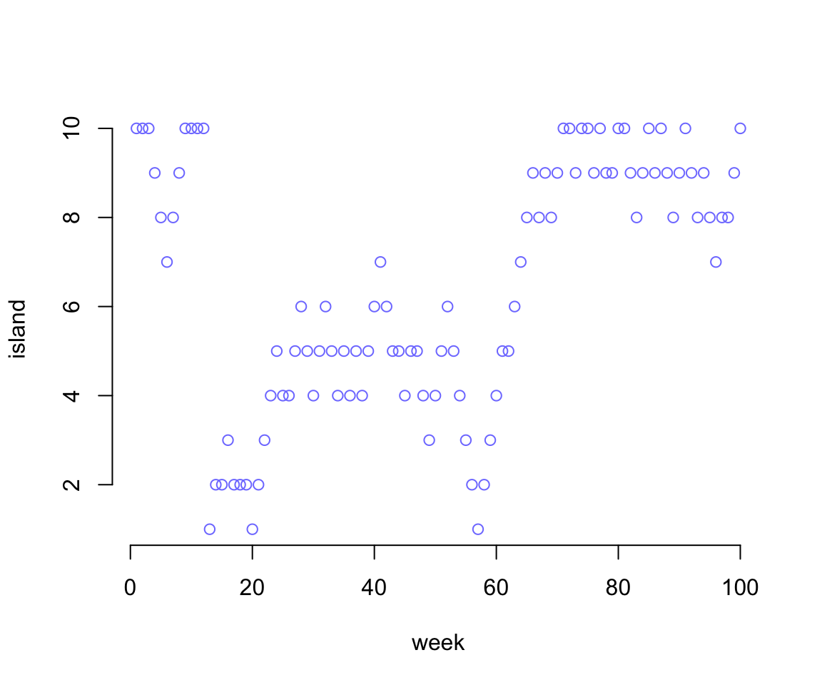
圖 52.1: Results of the king following the Metropolis algorithm. This figure shows the king’s current position (vertical axis) across weeks (horizontal axis). In any particular week, it’s nearly impossible to say where the king will be.
圖 52.1 告訴我們國王的行程幾乎看起來沒有任何規律性。但是事實上,如果你把全部100000個星期的行程總結一下,會神奇地發現國王在每個島嶼所呆的時間恰好都與其人口規模成相應的比例:
plot(table(positions),
     bty = "n",
     xlab = "island",
     ylab = "number of weeks stayed",
      col = rangi2)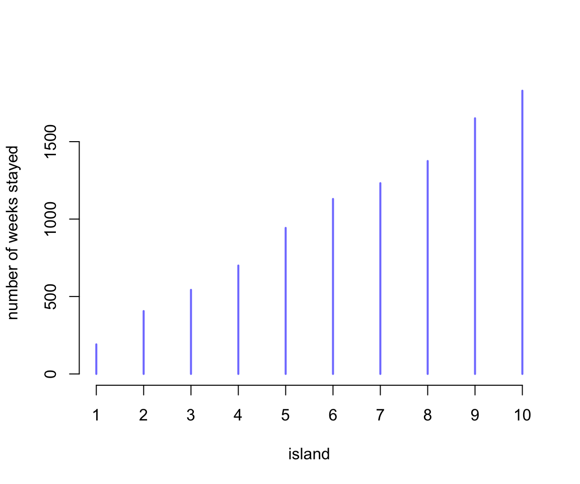
圖 52.2: Results of the king following the Metropolis algorithm. This figure shows the long-run behavior of the algorithm, as the time spent on each island turns out to be proportional to its population size.
52.2 Metropolis 演算法
上文中國王行程的例子其實是 Metropolis 演算法的一個特例,這就是一個簡單的馬可夫鏈蒙地卡羅過程。我們可以利用這個MCMC過程對模型給出的複雜的事後概率分佈樣本進行採樣。
- 例子中的“島嶼”,其實就是統計模型中的各種參數,它可以不必是離散型的,完全可以是連續型的變量。
- 每個島嶼的“人口規模”,其實是每個參數的事後概率分佈,在參數不同取值時的概率大小。
- 每個島嶼國王實際留駐的時間“週”,其實就是我們通過這個 Metropolis 演算法對事後概率分佈採集的樣本。
52.3 簡單的 HMC (Hamitonian Monte Carlo) ulam
這裏使用非洲大陸地理的數據 rugged,來作爲簡單的HMC過程的示範。
data("rugged")
d <- rugged
d$log_gdp <- log(d$rgdppc_2000)
dd <- d[ complete.cases(d$rgdppc_2000), ]
dd$log_gdp_std <- dd$log_gdp / mean(dd$log_gdp)
dd$rugged_std <- dd$rugged / max(dd$rugged)
dd$cid <- ifelse( dd$cont_africa == 1, 1, 2)
之前,我們使用二次方程近似法 quap() 時,加入了交互作用項的模型是:
m8.3 <- quap(
  alist(
    log_gdp_std ~ dnorm(mu, sigma),
    mu <- a[cid] + b[cid] * (rugged_std - 0.215) ,
    a[cid] ~ dnorm( 1, 0.1 ),
    b[cid] ~ dnorm( 0, 0.3 ),
    sigma ~ dexp( 1 )
  ), data = dd
)precis( m8.3, depth = 2 )## mean sd 5.5% 94.5%
## a[1] 0.88655682 0.0156750452 0.861505070 0.911608569
## a[2] 1.05057127 0.0099361951 1.034691314 1.066451232
## b[1] 0.13251798 0.0742015273 0.013929608 0.251106352
## b[2] -0.14263748 0.0547471324 -0.230133970 -0.055140987
## sigma 0.10948955 0.0059346769 0.100004789 0.118974309當我們準備使用 HMC 來採樣時,我們需要額外加以準備:
- 先處理所有需要中心化或者重新更改尺度的變量。
- 重新製作一個不含有多餘變量的數據集。(推薦)
dat_slim <- list(
  log_gdp_std = dd$log_gdp_std,
  rugged_std = dd$rugged_std,
  cid = as.integer(dd$cid)
)
str(dat_slim)
## List of 3
## $ log_gdp_std: num [1:170] 0.88 0.965 1.166 1.104 0.915 ...
## $ rugged_std : num [1:170] 0.138 0.553 0.124 0.125 0.433 ...
## $ cid : int [1:170] 1 2 2 2 2 2 2 2 2 1 ...準備好了數據之後,接下來,我們使用 Stan 進行事後分佈樣本採集:
m9.1 <- ulam(
  alist(
    log_gdp_std ~ dnorm( mu, sigma ),
    mu <- a[cid] + b[cid] * ( rugged_std - 0.215 ) ,
    a[cid] ~ dnorm(1, 0.1),
    b[cid] ~ dnorm(0, 0.3),
    sigma ~ dexp(1)
  ), data = dat_slim, chains = 1
)precis( m9.1, depth = 2 )## mean sd 5.5% 94.5% n_eff Rhat4
## a[1] 0.88762598 0.0158139609 0.859848549 0.911856753 697.68286 0.99811888
## a[2] 1.05074808 0.0103372479 1.035717029 1.066637227 777.02098 0.99808908
## b[1] 0.13473017 0.0752015577 0.018559852 0.261751292 769.03930 0.99849918
## b[2] -0.14209256 0.0535298779 -0.225545276 -0.058127179 823.03571 0.99870607
## sigma 0.11101502 0.0059144792 0.101778834 0.120212208 680.78693 0.99799968我們還可以使用多条採樣鏈,及使用多個計算機內核以平行計算提升效率:
m9.1 <- ulam(
  alist(
    log_gdp_std ~ dnorm( mu, sigma ),
    mu <- a[cid] + b[cid] * ( rugged_std - 0.215 ) ,
    a[cid] ~ dnorm(1, 0.1),
    b[cid] ~ dnorm(0, 0.3),
    sigma ~ dexp(1)
  ), data = dat_slim, chains = 4, cores = 4
)
## recompiling to avoid crashing R sessionshow( m9.1 )## Hamiltonian Monte Carlo approximation
## 2000 samples from 4 chains
##
## Sampling durations (seconds):
## warmup sample total
## chain:1 0.11 0.07 0.18
## chain:2 0.10 0.08 0.18
## chain:3 0.11 0.07 0.17
## chain:4 0.11 0.07 0.17
##
## Formula:
## log_gdp_std ~ dnorm(mu, sigma)
## mu <- a[cid] + b[cid] * (rugged_std - 0.215)
## a[cid] ~ dnorm(1, 0.1)
## b[cid] ~ dnorm(0, 0.3)
## sigma ~ dexp(1)precis( m9.1 , depth = 2)## mean sd 5.5% 94.5% n_eff Rhat4
## a[1] 0.88674306 0.0156563425 0.861586947 0.911396112 2903.2637 0.99990676
## a[2] 1.05027714 0.0099248637 1.033960001 1.065427772 2879.2357 1.00061580
## b[1] 0.13081462 0.0762146077 0.012007032 0.251835824 2377.3737 0.99927176
## b[2] -0.14259349 0.0571381311 -0.230158554 -0.048035652 2930.1460 0.99966040
## sigma 0.11147787 0.0059532340 0.102428961 0.121188453 2456.4643 1.00007763除了使用 traceplot() 來進行診斷給出軌跡圖之外:
traceplot(m9.1)## [1] 1000
## [1] 1
## [1] 1000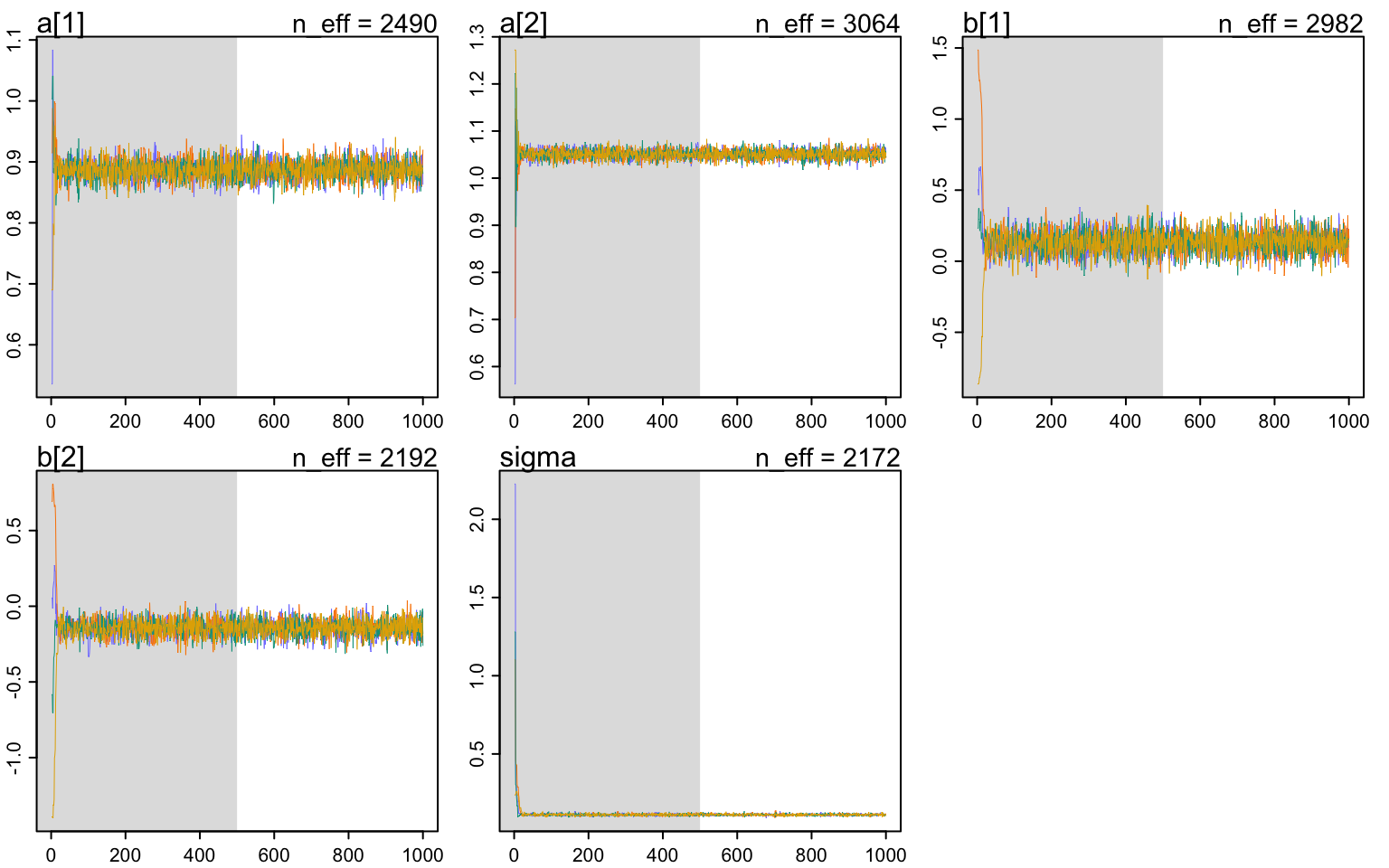
圖 52.3: Trace plot of the Markov chain from the ruggedness model, m9.1. (Gray region is warmup)
還可以使用 trunkplot() 繪製 軌跡排序圖 (trace rank plot)。
trankplot( m9.1 )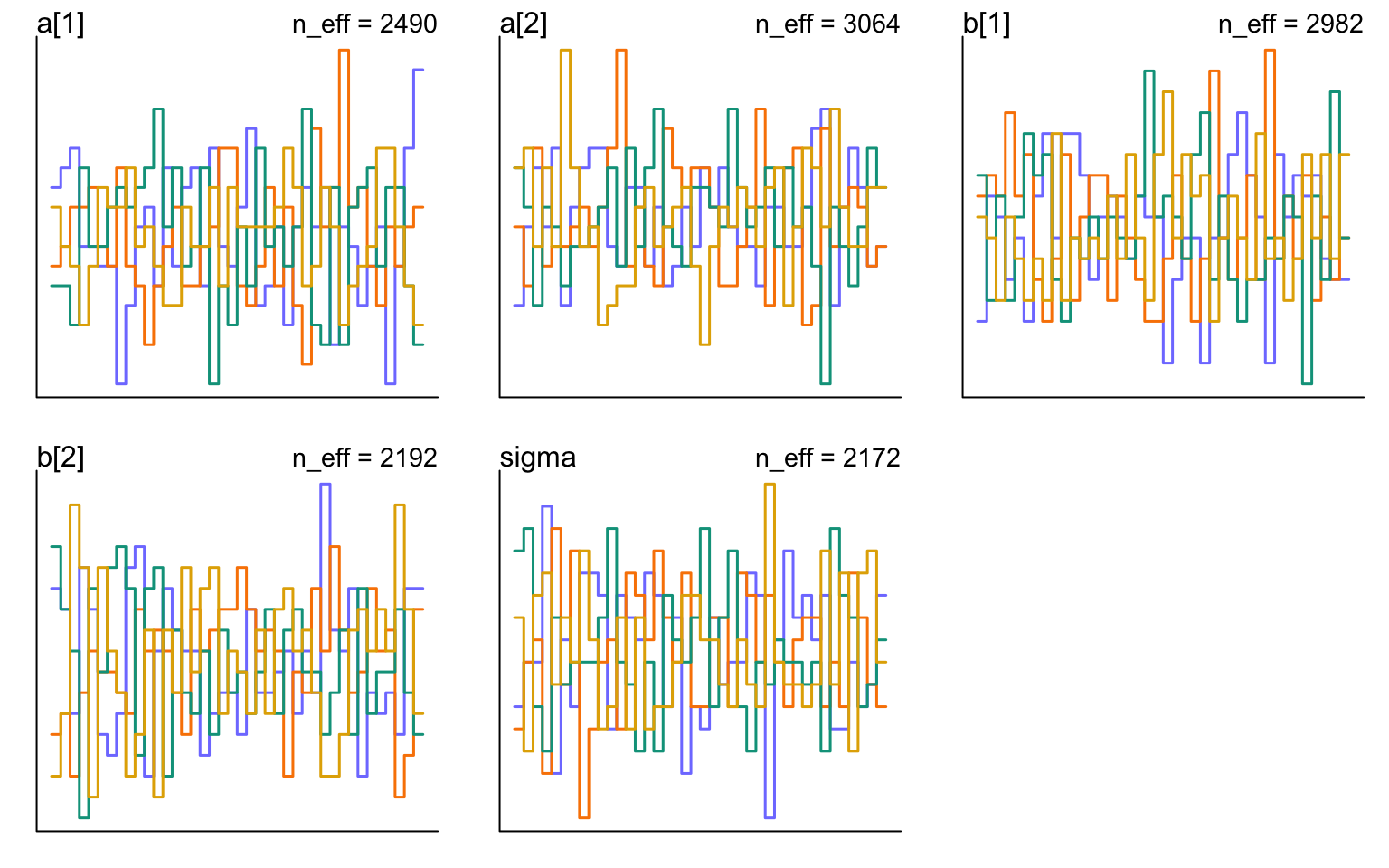
圖 52.4: Trunk plot of the Markov chain from the ruggedness model, m9.1.
使用 stancode() 可以閱讀計算機自動生成的 Stan 代碼:
stancode(m9.1)## data{
## vector[170] log_gdp_std;
## vector[170] rugged_std;
## int cid[170];
## }
## parameters{
## vector[2] a;
## vector[2] b;
## real<lower=0> sigma;
## }
## model{
## vector[170] mu;
## sigma ~ exponential( 1 );
## b ~ normal( 0 , 0.3 );
## a ~ normal( 1 , 0.1 );
## for ( i in 1:170 ) {
## mu[i] = a[cid[i]] + b[cid[i]] * (rugged_std[i] - 0.215);
## }
## log_gdp_std ~ normal( mu , sigma );
## }52.4 調教你的模型
有些模型給出的事後概率密度十分的寬且不準確,這常常是由於不加思索地給予所謂的“無信息先驗概率分佈”,也就是常見的平先驗概率分佈 (flat priors)。你可能會發現它給出的事後樣本採集鏈十分的野蠻,一會兒非常大,一會兒非常地小。下面是一個最簡單的例子,它用於計算兩個來自高斯分佈的觀察值 -1,和 1 的事後均值和標準差,使用的就是典型的平分佈作爲先驗概率分佈:
y <- c(-1, 1)
set.seed(11)
m9.2 <- ulam(
  alist(
    y ~ dnorm( mu, sigma ),
    mu <- alpha,
    alpha ~ dnorm( 0 , 1000 ),
    sigma ~ dexp(0.0001)
  ), data  = list(y = y), chains = 3
)
## Warning: There were 82 divergent transitions after warmup. See
## http://mc-stan.org/misc/warnings.html#divergent-transitions-after-warmup
## to find out why this is a problem and how to eliminate them.## Warning: Examine the pairs() plot to diagnose sampling problems## Warning: The largest R-hat is 1.07, indicating chains have not mixed.
## Running the chains for more iterations may help. See
## http://mc-stan.org/misc/warnings.html#r-hat## Warning: Bulk Effective Samples Size (ESS) is too low, indicating posterior means and medians may be unreliable.
## Running the chains for more iterations may help. See
## http://mc-stan.org/misc/warnings.html#bulk-ess## Warning: Tail Effective Samples Size (ESS) is too low, indicating posterior variances and tail quantiles may be unreliable.
## Running the chains for more iterations may help. See
## http://mc-stan.org/misc/warnings.html#tail-essprecis(m9.2)## mean sd 5.5% 94.5% n_eff Rhat4
## alpha 9.166007 345.61898 -437.590250 520.93025 102.84571 1.0283245
## sigma 620.035602 1514.59848 18.534647 2518.88736 198.57399 1.0384214你會看見你的計算機給出的結果非常的奇怪,且有警報提示可能計算出錯。上述結果肯定是不正常的,因為觀察值 -1,和 1 的平均值應該是 0 。你看上面的結果給出的可信區間也是多麼的荒謬。可用的有效樣本量也是小的可憐。你可以看看它的軌跡圖,和軌跡排序圖是多麼地糟糕:
traceplot(m9.2)## [1] 1000
## [1] 1
## [1] 1000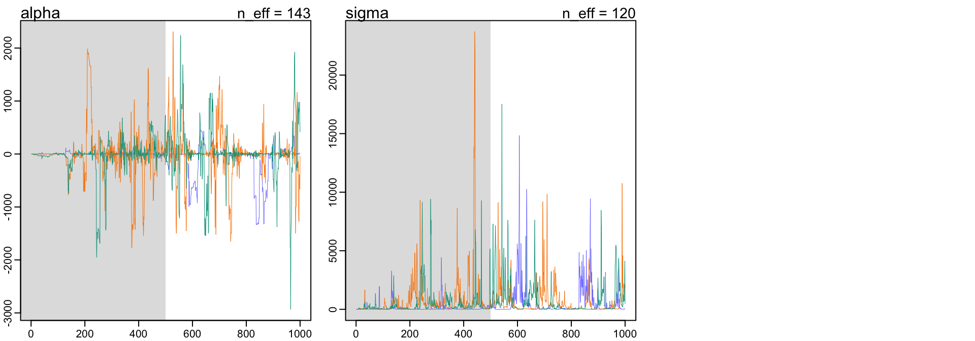
圖 52.5: Diagnosing trace plot from three trains by model m9.2. These chains are not healthy.
trankplot(m9.2)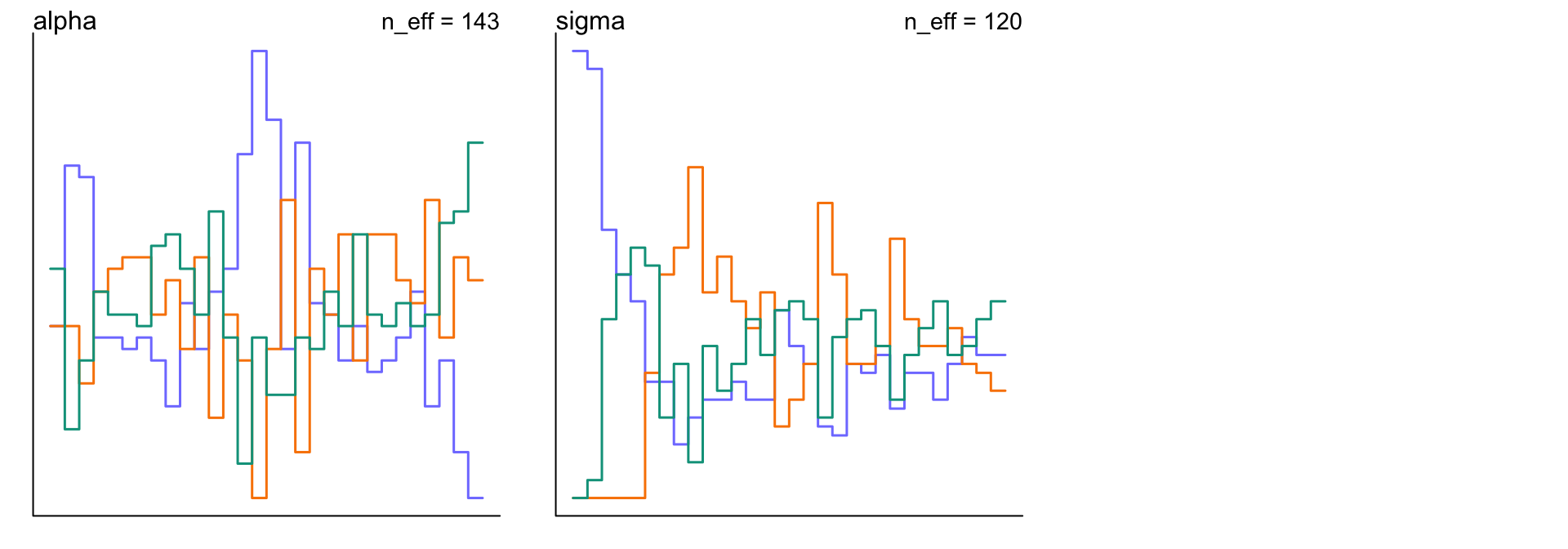
圖 52.6: Diagnosing trankplot from three chains by model 9.2. These chains are not healthy.
讓我們把模型修改成一個微調了先驗概率分佈的模型:
\[ \begin{aligned} y_i & \sim \text{Normal}(\mu, \sigma) \\ \mu & = \alpha \\ \color{red}{\alpha} &\; \color{red}{\sim \text{Normal}(1, 10)} \\ \color{red}{\sigma} &\; \color{red}{\sim \text{Exponential}(1)} \end{aligned} \]
我們僅僅是給均值,和對應的標準差增加了一點點比平概率分佈多一些信息的分佈。於是這個模型可以變成:
set.seed(11)
m9.3 <- ulam(
  alist(
    y ~ dnorm( mu, sigma ),
    mu <- alpha,
    alpha ~ dnorm(1, 10),
    sigma ~ dexp(1)
  ), data = list(y = y), chains = 3
)
## Warning: Tail Effective Samples Size (ESS) is too low, indicating posterior variances and tail quantiles may be unreliable.
## Running the chains for more iterations may help. See
## http://mc-stan.org/misc/warnings.html#tail-essprecis(m9.3)## mean sd 5.5% 94.5% n_eff Rhat4
## alpha 0.093687723 1.29168718 -1.58673258 2.2827566 294.92386 1.0059930
## sigma 1.572429387 0.92452697 0.69366299 3.0924262 254.86055 1.0037293可以看見,調教了一點點的先驗概率分佈之後給出的事後概率分佈估計就變得合理許多了。新的模型的軌跡圖和軌跡排序圖也變得合理許多:
traceplot(m9.3)## [1] 1000
## [1] 1
## [1] 1000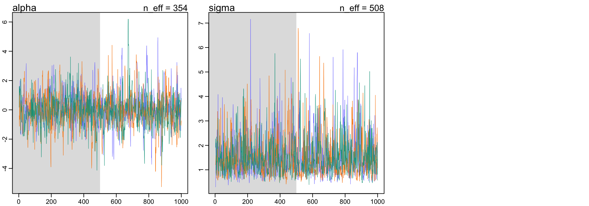
圖 52.7: Diagnosing trace plot from three trains by model m9.3. These chains are much better. Adding weakly informative priors in m9.3 clears up the condition.
trankplot(m9.3)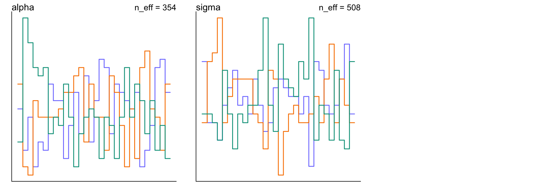
圖 52.8: Diagnosing trank plot from three trains by model m9.3. These chains are much better. Adding weakly informative priors in m9.3 clears up the condition.
可以看到對先驗概率分佈稍微增加一些微弱的信息之後,即便只有兩個觀察變量的數據給出的似然 likelihood 也已經遠遠把先驗概率的信息給掩蓋掉了,我們給出的先驗概率的均值是1,但是觀察數據兩個 -1 和 1 的均值是 0。
52.4.1 無法被確認的參數 non-identifiable parameters
之前我們就遇見了參數共線性給模型造成的麻煩 (Chapter 49.1)。這裏我們來觀察一下共線性變量造成的參數無法被估計的時候,MCMC給出的結果和預警會是怎樣的:
- 我們先從標準正(常)態分佈中隨機抽取100個觀察數據;
set.seed(41)
y <- rnorm(100, mean = 0, sd = 1)- 我們“錯誤地”使用下面的模型;
\[ \begin{aligned} y_i & \sim \text{Normal}(\mu, \sigma) \\ \mu & = \alpha_1 + \alpha_2 \\ \alpha_1 & \sim \text{Normal}(0, 1000) \\ \alpha_2 & \sim \text{Normal}(0, 1000) \\ \sigma & \sim \text{Exponential}(1) \end{aligned} \]
上述模型中的線性回歸模型,包含了兩個參數 \(\alpha_1, \alpha_2\) 他們是無法被估計的,但是他們的和,是可以被估計的,且由於我們先從正(常)態分佈中採集的觀察數據樣本,我們知道這個和應該在 0 附近不會太遠。
- 下面的代碼是上述模型的翻譯,這時 Stan 運行的時間會較長;
set.seed(384)
m9.4 <- ulam(
  alist(
    y ~ dnorm( mu, sigma ),
    mu <- a1 + a2,
    a1 ~ dnorm( 0, 1000 ),
    a2 ~ dnorm( 0, 1000 ),
    sigma ~ dexp(1)
  ), data = list(y = y), chains = 3
)
## Warning: There were 1164 transitions after warmup that exceeded the maximum treedepth. Increase max_treedepth above 10. See
## http://mc-stan.org/misc/warnings.html#maximum-treedepth-exceeded## Warning: Examine the pairs() plot to diagnose sampling problems## Warning: The largest R-hat is 2.44, indicating chains have not mixed.
## Running the chains for more iterations may help. See
## http://mc-stan.org/misc/warnings.html#r-hat## Warning: Bulk Effective Samples Size (ESS) is too low, indicating posterior means and medians may be unreliable.
## Running the chains for more iterations may help. See
## http://mc-stan.org/misc/warnings.html#bulk-ess## Warning: Tail Effective Samples Size (ESS) is too low, indicating posterior variances and tail quantiles may be unreliable.
## Running the chains for more iterations may help. See
## http://mc-stan.org/misc/warnings.html#tail-essprecis(m9.4)## mean sd 5.5% 94.5% n_eff Rhat4
## a1 -373.1298702 423.519109700 -1163.04089447 230.1858572 2.2415949 2.5908165
## a2 373.3204789 423.515716467 -230.04440214 1163.3392189 2.2415936 2.5908078
## sigma 1.0688708 0.087993227 0.94201267 1.2186705 3.2917766 1.5882462看上面的模型給出的估計是多麼的可怕。有效樣本量竟然只有個位數。\(\hat{R}\) 的估計值也是大得驚人。a1, a2 的取值距離0都十分遙遠,標準差也大得驚人,且它們之和十分接近 0 。這就是兩個參數之和可求,但是他們各自卻有無窮解的實例。你觀察一下上述模型的軌跡圖:
traceplot(m9.4)## [1] 1000
## [1] 1
## [1] 1000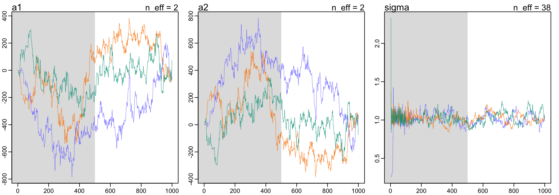
圖 52.9: Diagnosing trace plot from three trains by model m9.4. These chains are unhealthy, and wandering between different values and unstable. You cannot use these samples.
trankplot(m9.4)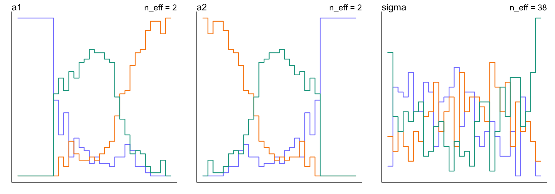
圖 52.10: Diagnosing trank plot from three trains by model m9.5. These chains are unhealthy, and wandering between different values and unstable. You cannot use these samples.
同樣地,對先驗概率分佈加以調整之後,有助於我們的模型事後樣本的採集。
set.seed(384)
m9.5 <- ulam(
  alist(
    y ~ dnorm( mu, sigma ),
    mu <- a1 + a2,
    a1 ~ dnorm( 0, 10 ),
    a2 ~ dnorm( 0, 10 ),
    sigma ~ dexp(1)
  ), data = list(y = y), chains = 3
)
## Warning: Bulk Effective Samples Size (ESS) is too low, indicating posterior means and medians may be unreliable.
## Running the chains for more iterations may help. See
## http://mc-stan.org/misc/warnings.html#bulk-ess## Warning: Tail Effective Samples Size (ESS) is too low, indicating posterior variances and tail quantiles may be unreliable.
## Running the chains for more iterations may help. See
## http://mc-stan.org/misc/warnings.html#tail-essprecis(m9.5)## mean sd 5.5% 94.5% n_eff Rhat4
## a1 0.65881633 7.530671388 -10.99718160 12.7162930 255.63033 1.0081006
## a2 -0.46679886 7.531880308 -12.56272791 11.2457817 254.94687 1.0080639
## sigma 1.03045997 0.077208825 0.91167928 1.1619185 445.68349 1.0015433這時 m9.5 運行的速度提升了很多,且 a1, a2 的事後樣本估計比之前的 m9.4 要良好得多。軌跡圖和軌跡排序圖也要改善了很多:
traceplot(m9.5)## [1] 1000
## [1] 1
## [1] 1000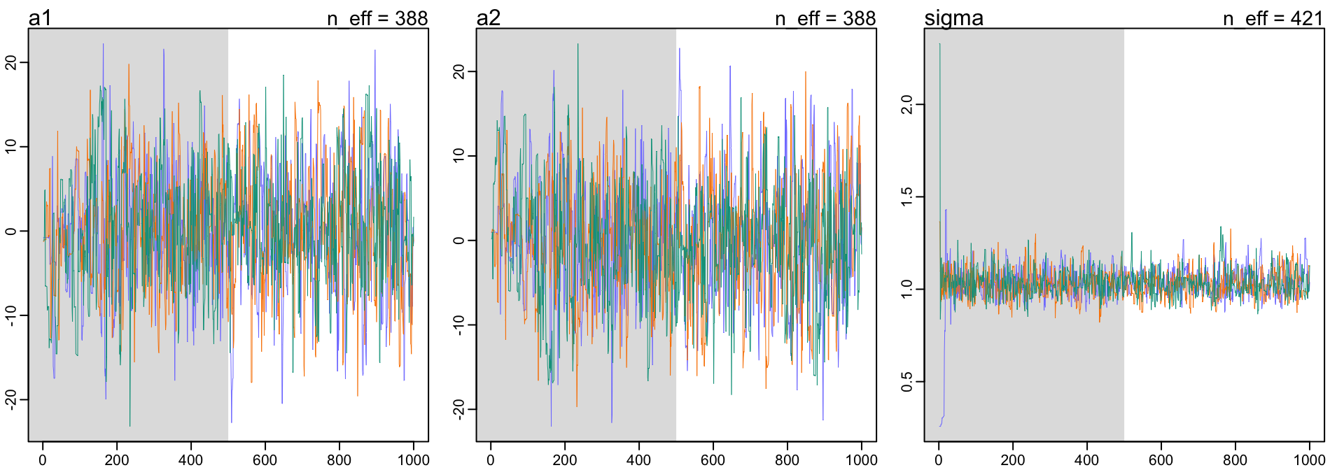
圖 52.11: Diagnosing trace plot from three trains by model m9.5. These chains are much better with the same model but weakly informative priors
trankplot(m9.5)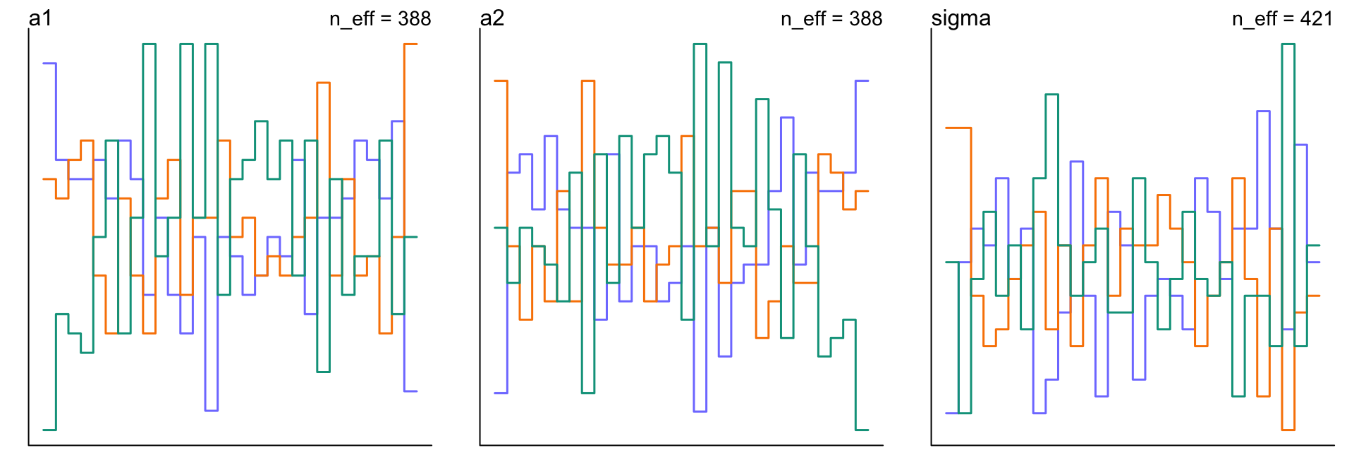
圖 52.12: Diagnosing trank plot from three trains by model m9.5. These chains are much better with the same model but weakly informative priors
如果一個模型,它的事後概率分佈的採樣過程太過於漫長,那麼它很可能就是由於有些參數出現了無法被估計的現象。請試着給它的先驗概率分佈加一些較爲微弱的信息以改善模型的樣本採集過程。儘量不要使用完全無信息的平概率分佈作爲先驗概率分佈。