第 46 章 簡單線型回歸模型 - 地心說模型 Linear regression is the geocentric model of applied statistics
這裡的簡單筆記來自經典教學書 Statistical Rethinking。
46.1 為什麼正(常)態分佈是正常的 why normal distribution is normal?
- Keep in mind that using a model is not equivalent to swearing an oath on it. The golem is your servant, not the other way around.
- Richard McElreath
概率分佈如果是離散型的,如二項分佈,描述它的分佈函數被叫做概率質量函數 (probability mass functions)。當概率分佈是連續型的,如正(常)態/高斯分佈,描述它的分佈函數被叫做概率密度函數 (probability density functions)。概率密度本身的取值是可以大於1的,如:
dnorm(0, 0, 0.1) # mean = 0, sd = 0.1## [1] 3.9894228是讓 R 幫助我們計算 \(p(0 | 0, (\sqrt{0.1})^2)\) 的取值。其結果差不多要等於4。這並沒有出錯,概率密度的概念其實是累積概率的增長速率 (the rate of change in cumulative probability)。所以在概率密度函數的平滑曲線上,累積概率增加的越快的區間,它的增長速率,也就是概率密度很容易超過1。但是,概率密度函數的曲線下面積,則永遠不可能超過1。
46.2 身高的高斯模型 Gaussian model of height
# library(rethinking)
data("Howell1")

d <- Howell1
str(d)
## 'data.frame': 544 obs. of 4 variables:
## $ height: num 152 140 137 157 145 ...
## $ weight: num 47.8 36.5 31.9 53 41.3 ...
## $ age : num 63 63 65 41 51 35 32 27 19 54 ...
## $ male : int 1 0 0 1 0 1 0 1 0 1 ...precis(d)## mean sd 5.5% 94.5% histogram
## height 138.26359632 27.60244764 81.1085500 165.735000 ▁▁▁▁▁▁▁▂▁▇▇▅▁
## weight 35.61061759 14.71917818 9.3607214 54.502894 ▁▂▃▂▂▂▂▅▇▇▃▂▁
## age 29.34439338 20.74688822 1.0000000 66.135000 ▇▅▅▃▅▂▂▁▁
## male 0.47242647 0.49969861 0.0000000 1.000000 ▇▁▁▁▁▁▁▁▁▇# filter out non-adults
d2 <- d[ d$age >= 18, ]寫下身高的模型,
\[ \begin{aligned} h_i & \sim \text{Normal}(\mu, \sigma) &\text{ [Likelihood]} \\ \mu & \sim \text{Normal}(178, 20) &\text{ [prior for } \mu] \\ \sigma & \sim \text{Uniform}(0, 50) &\text{ [prior for } \sigma]\\ \end{aligned} \]
觀察一下我們設定的先驗概率分佈的形狀:
curve( dnorm( x, 178, 20), from = 100, to = 250, xlab = ~mu)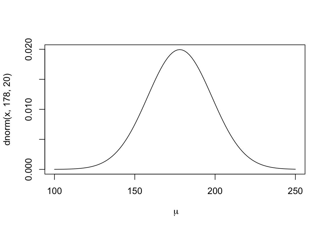
圖 46.1: The shape for prior distribution of the mean.
curve( dunif( x, 0, 50), from = -10, to = 60, xlab = ~sigma)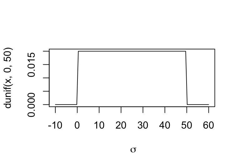
圖 46.2: The shape for prior distribution of the standard deviation.
當你選定了參數 \(h, \mu, \sigma\) 的先驗概率分佈時,你其實同時選定了他們的聯合分佈 (joint distribution)。從這個聯合先驗概率分佈中採集一些樣本,可以輔助我們判斷選擇這樣的先驗概率分佈是否是合適/不壞的。
sample_mu <- rnorm(10000, 178, 20)
sample_sigma <- runif(10000, 0, 50)
prior_h <- rnorm(10000, sample_mu, sample_sigma)
dens( prior_h )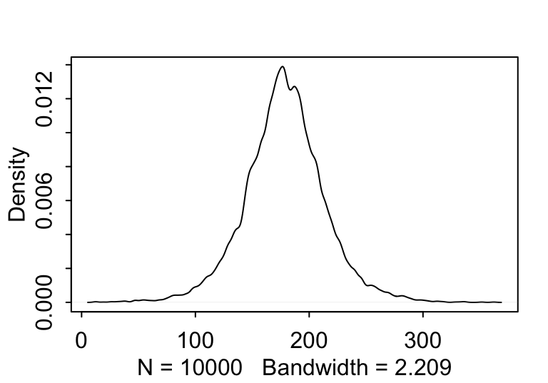
圖 46.3: The shape for samplings from prior distribution of the height generated from the joint distrition chosen for the mean and standard deviation.
看起來身高的先驗概率分佈似乎合乎常理,可以暫且認為均值和標準差的先驗概率選擇並不太糟糕。
當你刻意去選擇更加寬泛的先驗概率分佈給均值時,可能導致不合理的數據出現。如下圖 46.4 中顯示的那樣,當刻意給身高的均值 \(\mu\) 賦予更加“不含信息”,或者模糊的先驗概率 \(\text{Normal}(178, 100)\),時給出的身高的先驗概率分佈中出現了不少身高為負數的情況,這就是不合理的先驗概率分佈。
sample_mu <- rnorm(10000, 178, 100)
prior_h <- rnorm(10000, sample_mu, sample_sigma)
dens( prior_h )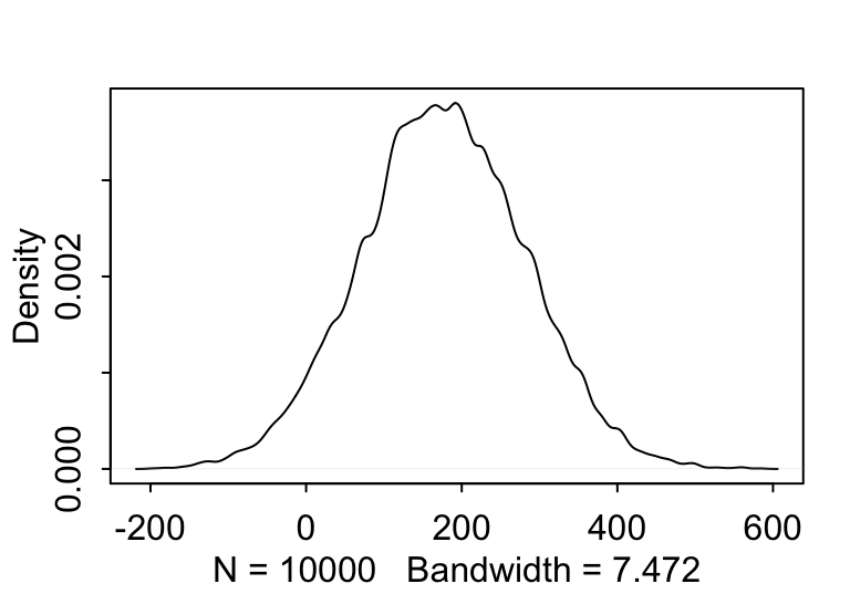
圖 46.4: The shape for samplings from prior distribution of the height generated from the joint distrition chosen for the mean and standard deviation, with flatter and less information prior for the mean (mu ~ N(178, 100)).
模型的貝葉斯定理表達式:
\[ \text{Pr}(\mu, \sigma | h) = \frac{\prod_i \text{Normal}(h_i|\mu, \sigma)\text{Normal}(\mu | 178, 20)\text{Uniform}(\sigma|0,50)}{\int\int \prod_i \text{Normal}(h_i|\mu, \sigma)\text{Normal}(\mu | 178, 20)\text{Uniform}(\sigma|0,50) d\mu d\sigma} \]
46.2.1 小方格估計法近似事後概率分佈
# 在 150 - 160 之間產生100個數據區間
mu_list <- seq( from = 150, to = 160, length.out = 100)

# 在 7-9 之間產生 100 個數據區間
sigma_list <- seq( from  = 7, to = 9, length.out = 100)

# 用上面生成的方差和均值交叉做出 10000 個均值和方差的數據格子
post <- expand.grid( mu = mu_list, sigma = sigma_list)

# 在對數尺度上用加法運算,會節約計算成本
post$LL <- sapply( 1:nrow(post), function(i) sum(
  dnorm( d2$height, post$mu[i], post$sigma[i], log = TRUE)
))

# 計算取對數下的事後概率分佈的分母部分
post$prod <- post$LL +
  dnorm( post$mu, 178, 20, log = TRUE) +
  dunif(post$sigma, 0, 50, log = TRUE)

# Scale all of the log-products by the maximum log-product

post$prob <- exp( post$prod - max(post$prod))
可以繪製簡單的事後均值,事後標準差的等高圖分佈,登高線本身使用上面代碼計算的身高的相對事後概率分佈。
contour_xyz( post$mu, post$sigma, post$prob)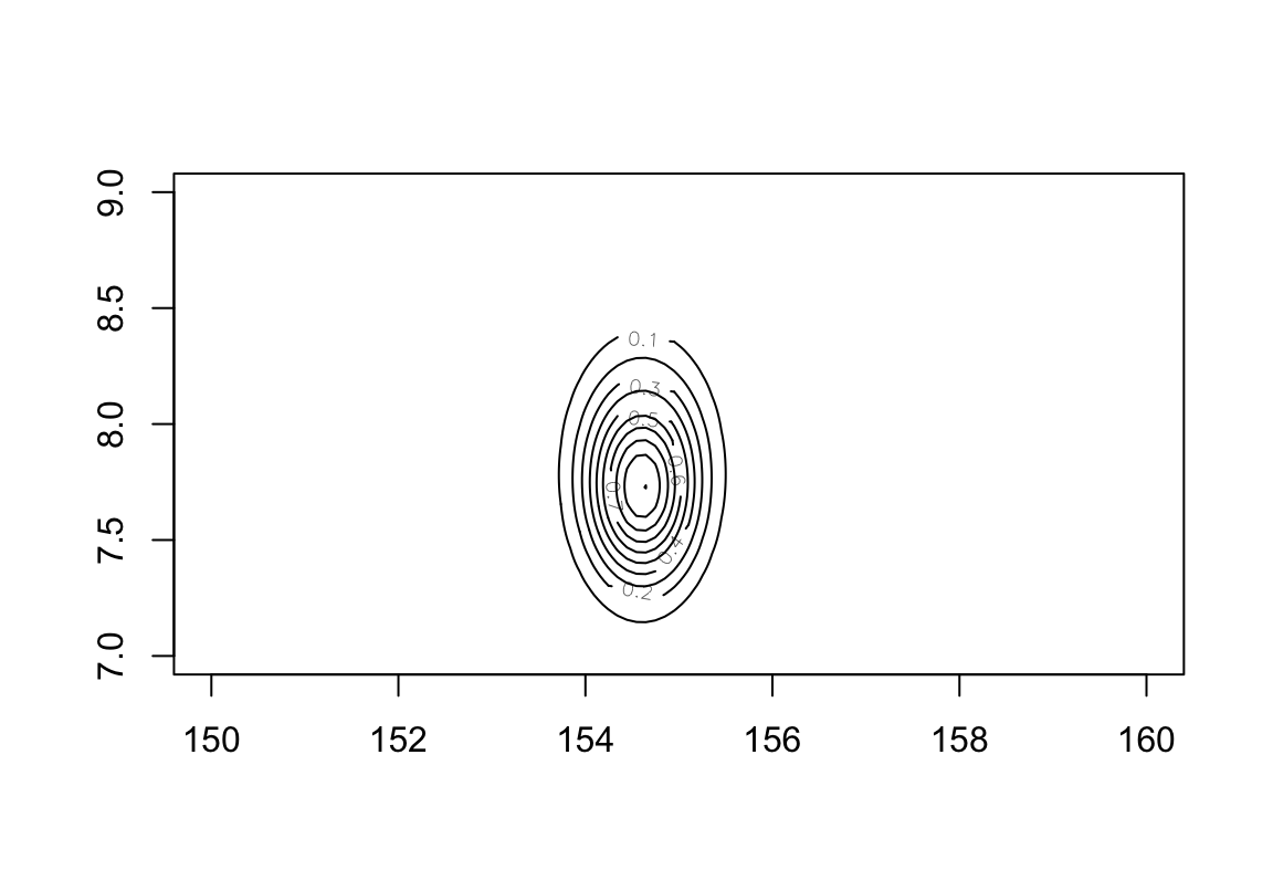
圖 46.5: Simple contour plot of the posterior means and standard deviations of height with relative posterior probability distribution.
image_xyz(post$mu, post$sigma, post$prob)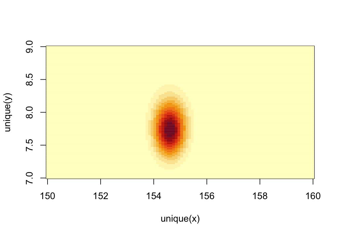
圖 46.6: Simple heat map plot of the posterior means and standard deviations of height with relative posterior probability distribution.
46.2.2 從計算獲得的事後概率分佈中採樣
sample.rows <- sample(1 : nrow(post), size = 10000, replace = TRUE,
                      prob = post$prob)
sample.mu <- post$mu[ sample.rows ]
sample.sigma <- post$sigma[ sample.rows]

plot(sample.mu, sample.sigma, cex = 0.7, pch = 16,
     col = col.alpha(rangi2, 0.2))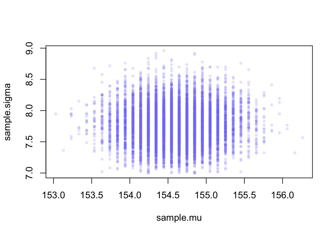
圖 46.7: Samples from the posterior distribution for the heights data.
dens(sample.mu)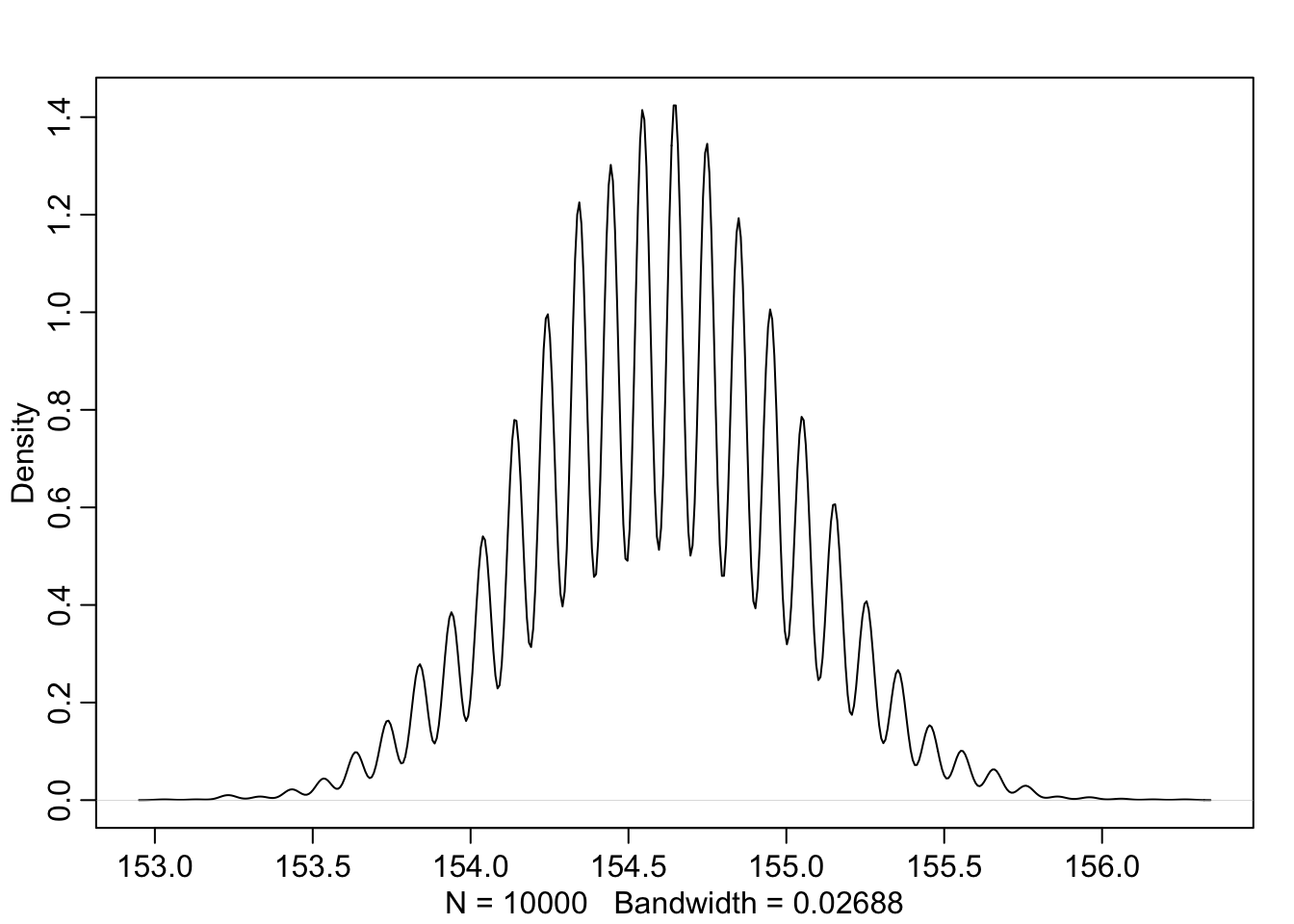
dens(sample.sigma)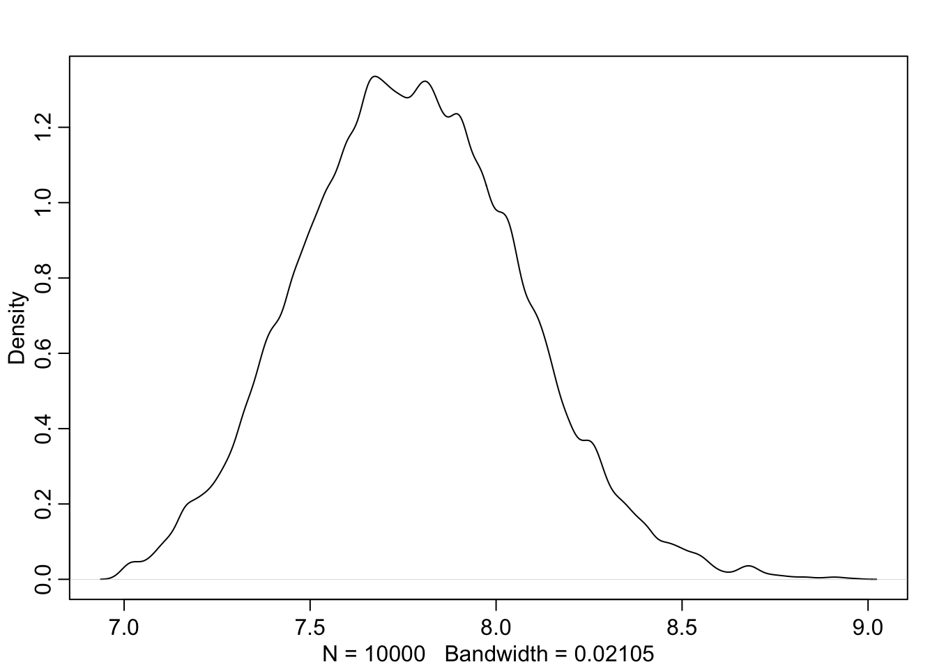
PI(sample.mu)## 5% 94%
## 153.93939 155.25253PI(sample.sigma)## 5% 94%
## 7.3232323 8.252525346.2.3 使用二次方程近似法
使用R語言定義我們的身高模型:
\[ \begin{aligned} h_i & \sim \text{Normal}(\mu, \sigma) &\text{ [Likelihood]} \\ \mu & \sim \text{Normal}(178, 20) &\text{ [prior for } \mu] \\ \sigma & \sim \text{Uniform}(0, 50) &\text{ [prior for } \sigma]\\ \end{aligned} \]
flist <- alist(
  height ~ dnorm( mu, sigma ),
  mu     ~ dnorm( 178, 20 ),
  sigma  ~ dunif( 0 , 50 )
)

m4.1 <- quap( flist, data = d2)

precis( m4.1 )
## mean sd 5.5% 94.5%
## mu 154.6069052 0.41197187 153.9484946 155.2653158
## sigma 7.7309053 0.29134573 7.2652786 8.1965321繪製該數據中身高曲線之間的關係圖:
# plot(d2$height, d2$weight)
ggplot(data = d2,
       aes(x = weight, y = height)) +
  geom_point(shape = 1, size = 2) +
  theme_bw() +
  theme(panel.grid = element_blank())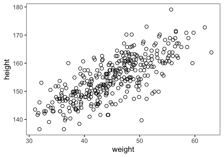
圖 46.8: Plot adults height against weight.
如何使用身高來做體重的預測變量,從而建立一個簡單線型回歸模型?
\[ \begin{aligned} h_i & \sim \text{Normal}(\mu_i, \sigma) & [\text{likelihood}]\\ \mu_i & = \alpha + \beta (x_i - \bar{x}) & [\text{linear model}]\\ \alpha & \sim \text{Normal}(178, 20) & [\text{prior for } \alpha]\\ \beta & \sim \text{Normal}(0, 10) & [\text{prior for } \beta]\\ \sigma & \sim \text{Uniform}(0, 50) & [\text{prior for } \sigma] \end{aligned} \]
46.2.4 關於 \(\beta\) 的先驗概率 Priors
代碼來自書中(P95 Rcode 4.38):
set.seed(2971)
N <- 100 #n number of simulation lines

a <- rnorm( N, 178, 20)
b <- rnorm( N, 0, 10)

plot( NULL, xlim = range(d2$weight) , ylim = c(-100, 400),
      xlab = "weight", ylab = "height")
abline( h = 0, lty = 2)
abline( h = 272, lty = 1, lwd = 0.5)
mtext("b ~ dnorm(0, 10)" )

xbar <- mean(d2$weight)

for ( i in 1:N) curve( a[i] + b[i]*(x - xbar) ,
  from = min(d2$weight), to = max(d2$weight), add = TRUE,
  col = col.alpha("black", 0.2)
  )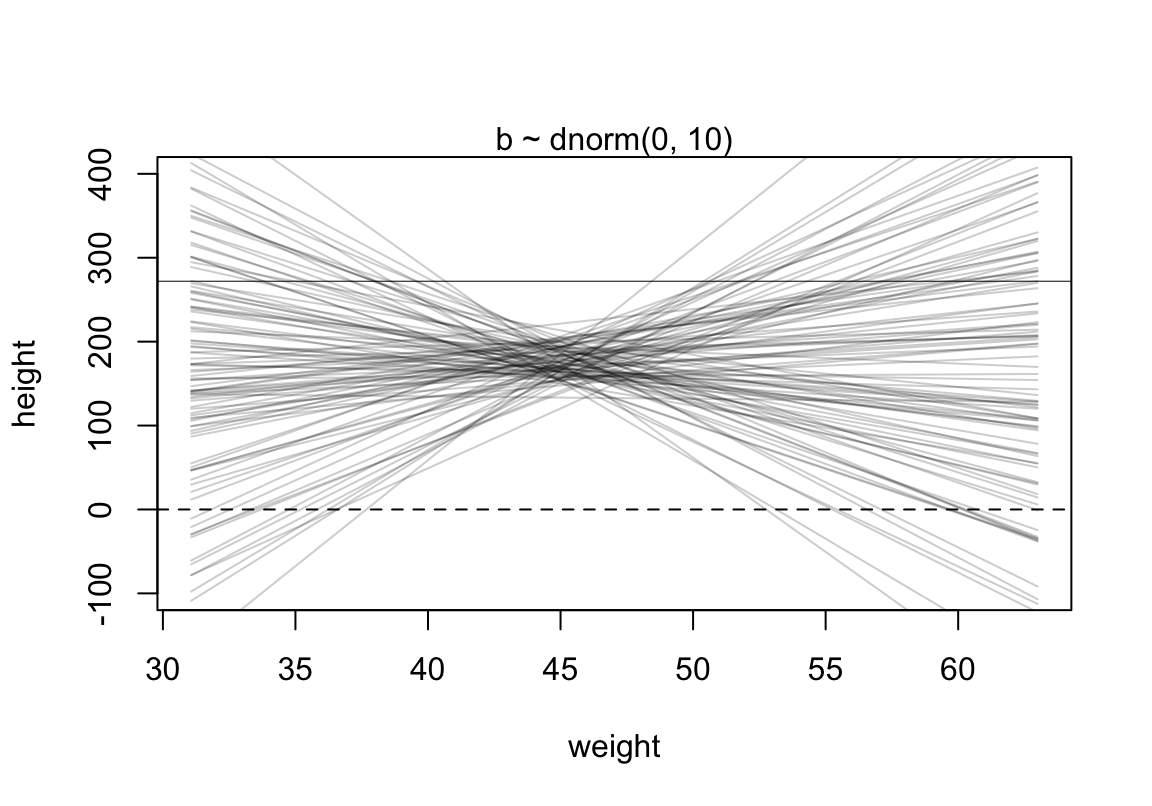
圖 46.9: Prior predictive simulation for the height and weight model. Simulation using the beta ~ N(0, 10) prior.
相同圖形使用 tidyverse 和 ggplot2 來製作(參考 Statistical rethinking with brms, ggplot2, and the tidyverse: Second edition:
set.seed(4)
# how many lines would you like?
n_lines <- 100

lines <-
  tibble(n = 1:n_lines,
         a = rnorm(n_lines, mean = 178, sd = 20),
         b = rnorm(n_lines, mean = 0,   sd = 10)) %>%
  tidyr::expand(tidyr::nesting(n, a, b), weight = range(d2$weight)) %>%
  mutate(height = a + b * (weight - mean(d2$weight)))

head(lines)
## # A tibble: 6 x 5
## n a b weight height
## <int> <dbl> <dbl> <dbl> <dbl>
## 1 1 182. 6.85 31.1 87.0
## 2 1 182. 6.85 63.0 306.
## 3 2 167. -1.15 31.1 183.
## 4 2 167. -1.15 63.0 146.
## 5 3 196. -3.56 31.1 245.
## 6 3 196. -3.56 63.0 132.lines %>%
ggplot(aes(x = weight, y = height, group = n)) +
geom_hline(yintercept = c(0, 272), linetype = 2:1, size = 1/3) +
geom_line(alpha = 1/10) +
coord_cartesian(ylim = c(-100, 400)) +
ggtitle("b ~ dnorm(0, 10)") +
theme_classic()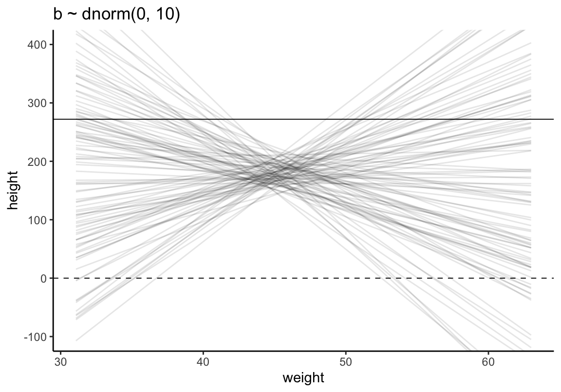
圖 46.10: Prior predictive simulation for the height and weight model. Simulation using the beta ~ N(0, 10) prior.
可見這樣的身高作為先驗概率明顯是不合理的,因為有大量的數據低於 0 cm,甚至於大於人類的極限身高272cm。如何將這個關於身高的先驗概率合理化呢?解決方法的一種是使用對數正(常)態分佈。對數正(常)態分佈,其實就是指,一組取了對數之後的數值服從正(常)態分佈。
\[ \beta \sim \text{Log-Normal}(0, 1) \]
# b <- rlnorm(10000, 0, 1)
# dens(b, xlim = c(0, 5), adj = 0.1)
set.seed(4)
tibble(b = rlnorm(10000, mean = 0, sd = 1)) %>%
  ggplot(aes(x = b)) +
  geom_density(fill = "grey70") +
  coord_cartesian(xlim = c(0, 5)) +
  theme_classic()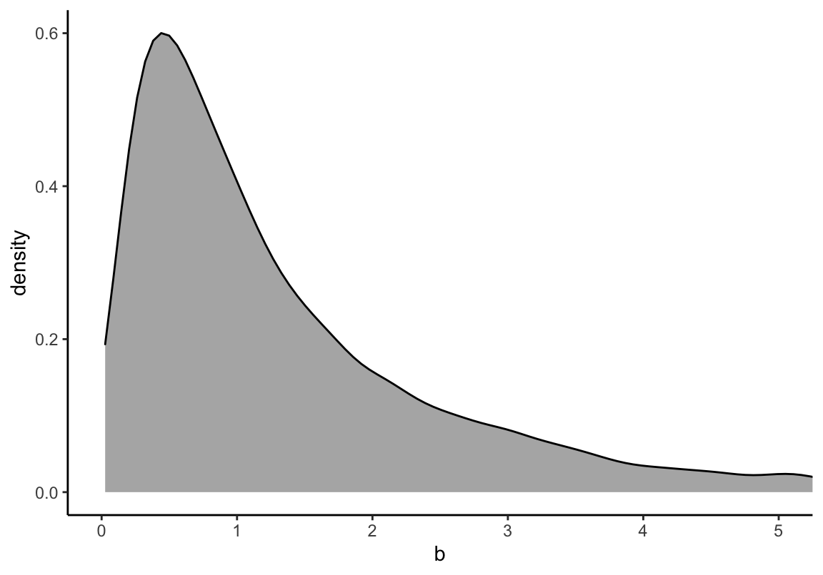
圖 46.11: The density shape for lognormal (0,1), it is the distribution whose logarithm is normally distributed.
我們還可以把採集的對數正(常)態分佈樣本取對數,和標準正(常)態分佈做一個圖形上的比較。
set.seed(4)

tibble(rnorm = rnorm(100000, mean = 0, sd = 1),
       `log(rlognorm)` = log(rlnorm(100000, mean = 0, sd = 1))) %>%
  pivot_longer(everything()) %>%
  ggplot(aes(x = value)) +
  geom_density(fill = "grey70") +
  coord_cartesian(xlim = c(-3, 3)) +
  theme_classic() +
  facet_wrap( ~ name, nrow = 2)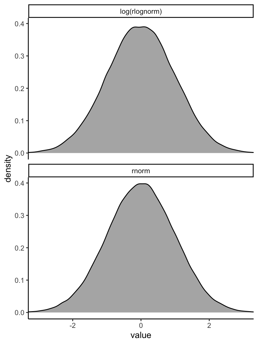
圖 46.12: The density shape for log(lognormal (0, 1)) and normal(0, 1), they are the same.
使用對數正(常)態分佈作為 \(\beta\) 的先驗概率分佈,試試看它給出的身高預測範圍大致是怎樣的。
set.seed(2971)
N <- 100 #n number of simulation lines

a <- rnorm( N, 178, 20)
# b <- rnorm( N, 0, 10)
b <- rlnorm( N, 0, 1)

plot( NULL, xlim = range(d2$weight) , ylim = c(-100, 400),
      xlab = "weight", ylab = "height")
abline( h = 0, lty = 2)
abline( h = 272, lty = 1, lwd = 0.5)
mtext("b ~ dlognorm(0, 1)" )

xbar <- mean(d2$weight)

for ( i in 1:N) curve( a[i] + b[i]*(x - xbar) ,
  from = min(d2$weight), to = max(d2$weight), add = TRUE,
  col = col.alpha("black", 0.2)
  )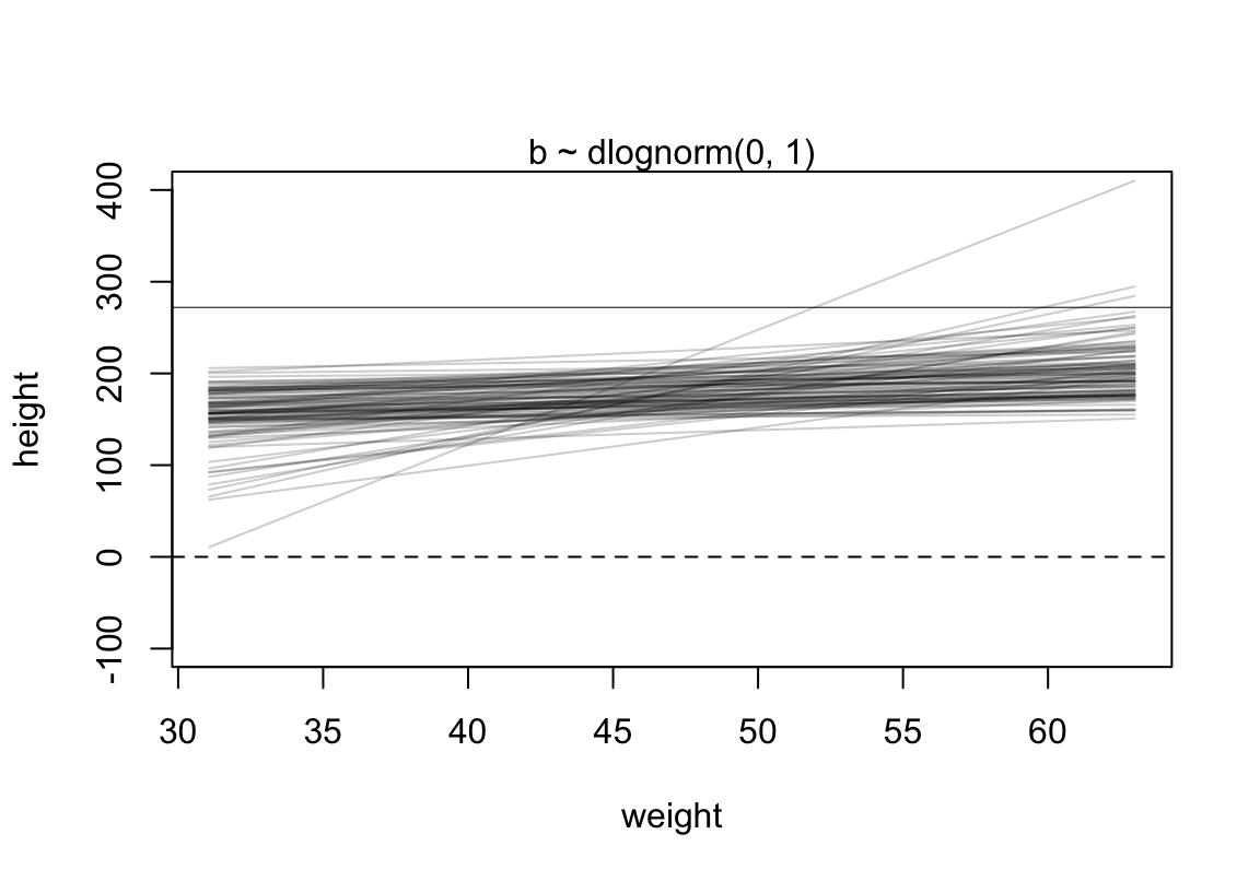
圖 46.13: Prior predictive simulation for the height and weight model. Simulation using the beta ~ log-normal(0, 1) prior, within much reasonable human ranges.
使用 ggplot2 做一邊相同的事。
# make a tibble to annotate the plot
Text <-
  tibble(weight = c(34, 43),
         height = c(0 - 25, 272 + 25),
         label  = c("Embryo", "World's tallest person (272 cm)"))

# simulate
set.seed(4)

tibble(n = 1:n_lines,
       a = rnorm(n_lines, mean = 178, sd = 20),
       b = rlnorm(n_lines, mean = 0, sd = 1)) %>%
  tidyr::expand(tidyr::nesting(n, a, b), weight = range(d2$weight)) %>%
  mutate(height = a + b * (weight - mean(d2$weight))) %>%

  # plot
  ggplot(aes(x = weight, y = height, group = n)) +
  geom_hline(yintercept = c(0, 272), linetype = 2:1, size = 1/3) +
  geom_line(alpha = 1/10) +
  annotate(geom = "text",
           x = c(34, 43), y = c(-25, 297),
           label = c("Embryo", "World's tallest person (272 cm)"),
           size = 5) +
  coord_cartesian(ylim = c(-100, 400)) +
  ggtitle("log(b) ~ dnorm(0, 1)") +
  theme_classic()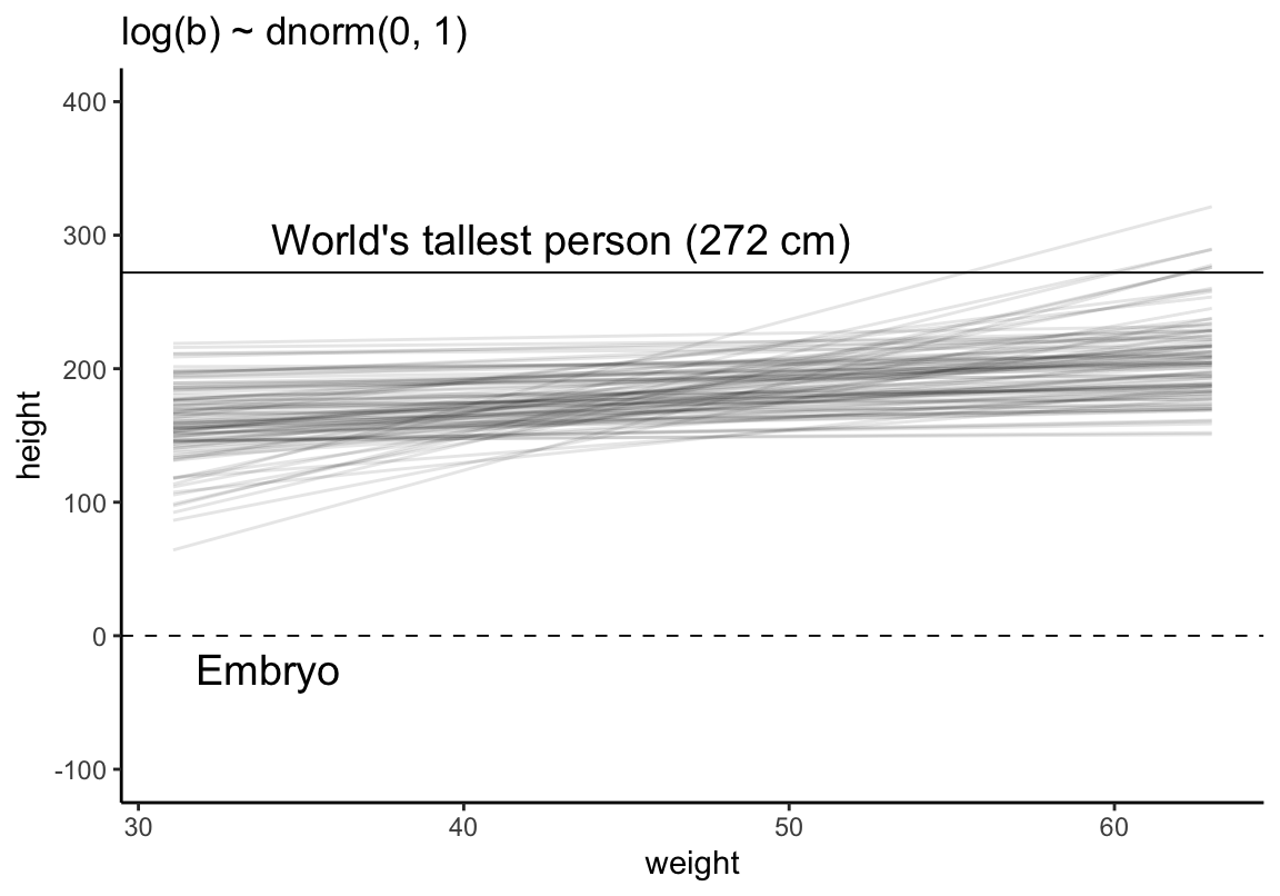
圖 46.14: Prior predictive simulation for the height and weight model. Simulation using the beta ~ log-normal(0, 1) prior, within much reasonable human ranges.
A serious problem in contemporary applied statistics is “p-hacking,” the practice of adjusting the model and the data to achieve a desired result. The desired result is usually a p-value less than 5%.
於是我們現在把修改了 \(\beta\) 的先驗概率分佈之後的模型定義:
\[ \begin{aligned} h_i & \sim \text{Normal}(\mu_i, \sigma) & [\text{likelihood}]\\ \mu_i & = \alpha + \beta (x_i - \bar{x}) & [\text{linear model}]\\ \alpha & \sim \text{Normal}(178, 20) & [\text{prior for } \alpha]\\ \beta & \sim \text{Log-Normal}(0, 1) & [\text{prior for } \beta]\\ \sigma & \sim \text{Uniform}(0, 50) & [\text{prior for } \sigma] \end{aligned} \]
於是用這個模型來獲取我們需要的事後概率分佈的方法就顯而易見了:
# define the average weight, x-bar
xbar <- mean(d2$weight)

# fit model

m4.3 <- quap(
  alist(
    height ~ dnorm( mu, sigma ),
    mu <- a + b * (weight - xbar),
    a ~ dnorm(178, 20),
    b ~ dlnorm(0, 1),
    sigma ~ dunif( 0, 50 )
  ), data = d2
)

precis(m4.3)
## mean sd 5.5% 94.5%
## a 154.60136213 0.270307731 154.16935816 155.0333661
## b 0.90328082 0.041923642 0.83627874 0.9702829
## sigma 5.07188225 0.191154909 4.76637978 5.3773847d2 <- d2 %>%
mutate(weight_c = weight - mean(weight))
b4.3 <-
brm(data = d2,
family = gaussian,
height ~ 1 + weight_c,
prior = c(prior(normal(178, 20), class = Intercept),
prior(lognormal(0, 1), class = b),
prior(uniform(0, 50), class = sigma)),
iter = 28000, warmup = 27000, chains = 4, cores = 4,
seed = 4)## Warning: It appears as if you have specified a lower bounded prior on a parameter that has no natural lower bound.
## If this is really what you want, please specify argument 'lb' of 'set_prior' appropriately.
## Warning occurred for prior
## b ~ lognormal(0, 1)## Warning: It appears as if you have specified an upper bounded prior on a parameter that has no natural upper bound.
## If this is really what you want, please specify argument 'ub' of 'set_prior' appropriately.
## Warning occurred for prior
## sigma ~ uniform(0, 50)b4.3## Family: gaussian
## Links: mu = identity; sigma = identity
## Formula: height ~ 1 + weight_c
## Data: d2 (Number of observations: 352)
## Samples: 4 chains, each with iter = 28000; warmup = 27000; thin = 1;
## total post-warmup samples = 4000
##
## Population-Level Effects:
## Estimate Est.Error l-95% CI u-95% CI Rhat Bulk_ESS Tail_ESS
## Intercept 154.60 0.27 154.08 155.14 1.00 4588 2820
## weight_c 0.90 0.04 0.83 0.99 1.01 614 673
##
## Family Specific Parameters:
## Estimate Est.Error l-95% CI u-95% CI Rhat Bulk_ESS Tail_ESS
## sigma 5.10 0.19 4.75 5.50 1.00 2719 2068
##
## Samples were drawn using sampling(NUTS). For each parameter, Bulk_ESS
## and Tail_ESS are effective sample size measures, and Rhat is the potential
## scale reduction factor on split chains (at convergence, Rhat = 1).觀察各個參數事後樣本之間的協方差 (covariances),幾乎可以忽略不計。
round( vcov(m4.3), 3)## a b sigma
## a 0.073 0.000 0.000
## b 0.000 0.002 0.000
## sigma 0.000 0.000 0.037posterior_samples(b4.3) %>%
dplyr::select(-lp__) %>%
cov() %>%
round(digits = 3)## b_Intercept b_weight_c sigma
## b_Intercept 0.076 0.000 0.000
## b_weight_c 0.000 0.002 0.000
## sigma 0.000 0.000 0.036pairs(m4.3)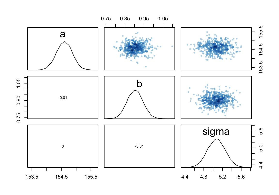
圖 46.15: Both marginal posteriors and the covariance.
pairs(b4.3)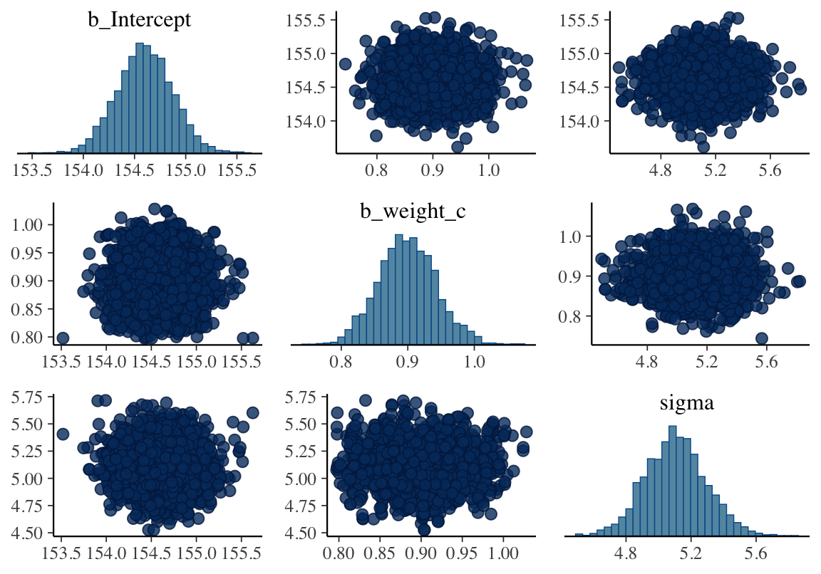
圖 46.16: Both marginal posteriors and the covariance.
繪製事後估計獲得的均值給出的回歸直線。
plot( height ~ weight, data = d2, col = rangi2)
post <- extract.samples(m4.3)
a_map <- mean(post$a)
b_map <- mean(post$b)
curve( a_map + b_map * (x - xbar), add = TRUE)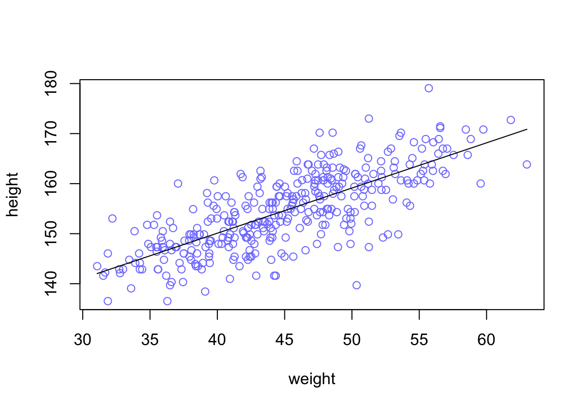
圖 46.17: Height in centimeters plotted against weight in kilograms, with the line at the posterior mean plotted in black.
ggplot2繪圖結果:
d2 %>%
ggplot(aes(x = weight_c, y = height)) +
geom_abline(intercept = fixef(b4.3)[1],
slope = fixef(b4.3)[2]) +
geom_point(shape = 1, size = 2, color = "royalblue") +
theme_classic()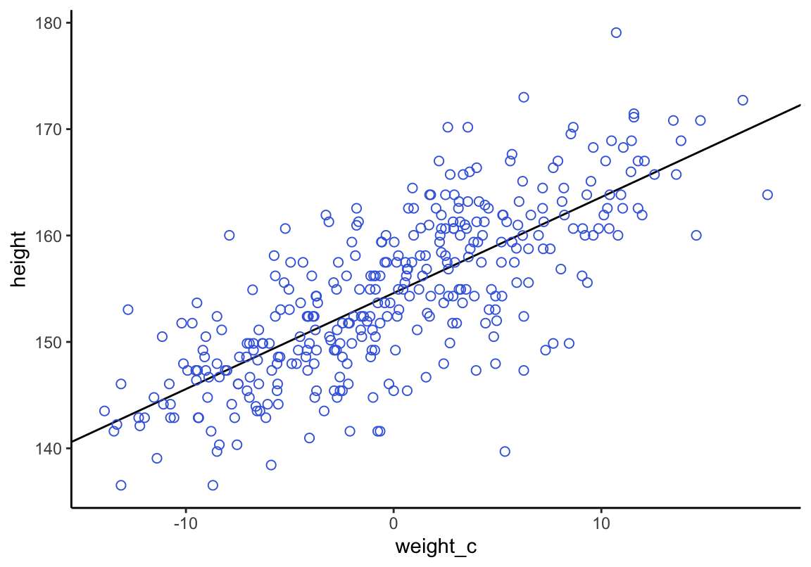
圖 46.18: Height in centimeters plotted against weight in kilograms, with the line at the posterior mean plotted in black.
為了顯示斜率和截距本身的不確定性,我們來從參數的事後聯合概率分佈中採集一些樣本出來做觀察:
post <- extract.samples( m4.3 )
post[1:5, ]## a b sigma
## 1 154.92100 0.84143701 5.0106009
## 2 155.01037 0.89948181 4.7643789
## 3 154.52622 0.86317290 5.1595400
## 4 154.36448 0.92057824 4.9611817
## 5 154.84028 0.96997643 4.9353836postb <- posterior_samples(b4.3)
postb %>%
slice(1:5)## b_Intercept b_weight_c sigma lp__
## 1 154.03954 0.88831753 5.0198152 -1081.0403
## 2 155.00645 0.88138939 5.1495396 -1080.0080
## 3 154.26479 0.86416946 5.2009147 -1080.0661
## 4 154.44802 0.91498529 4.9565292 -1079.1431
## 5 154.70723 0.91765800 5.1903559 -1079.0141這些 a, b 的無數配對,就是該線型回歸給出的事後回歸線的截距和斜率的無數的組合,每一個組合,是一條事後回歸直線。這些事後截距和事後斜率的均值,是圖 46.18 和 46.17 中的那條事後均值提供的直線。事實上,這些截距和斜率本身的不確定性才是更加值得關注的。
下面的計算過程是先使用 d2 數據中前10個人的身高體重做相同的事後回歸直線分析,然後逐漸增加數據量,你會觀察到這些事後斜率和事後截距的不確定性在發生的一個動態變化:
N <- 10
dN <- d2[1:N, ]
mN <- quap(
alist(
height ~ dnorm( mu, sigma ),
mu <- a + b*(weight - mean(weight)),
a ~ dnorm( 178, 20 ),
b ~ dlnorm( 0, 1 ),
sigma ~ dunif( 0, 50 )
), data = dN
)接下來繪製 mN 模型中給出的事後回歸直線的一部分:
# extract 20 samples from the posterior
post <- extract.samples( mN, n = 20)
# display raw data and sample size
plot(dN$weight, dN$height,
xlim = range(d2$weight), ylim = range(d2$height),
col = rangi2, xlab = "weight", ylab = "height")
mtext(concat( "N = ", N))
# plot the lines with transparency
for ( i in 1:20)
curve( post$a[i] + post$b[i] * (x - mean(dN$weight)),
col = col.alpha("black", 0.3), add = TRUE)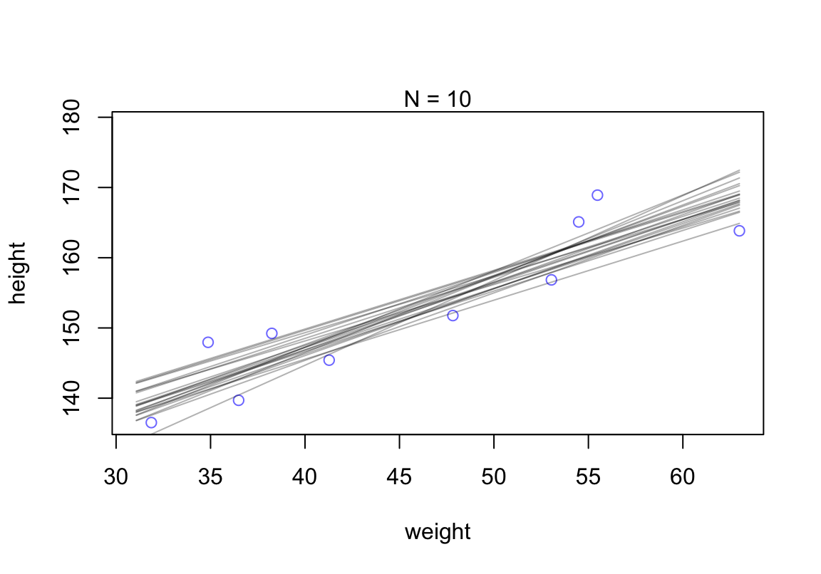
圖 46.19: Samples from the quadratic approximate posterior distribution for the height/weight model with 20 samples of data. 20 Lines sampled from the posterior distribution.
增加樣本量,你只需要修改上述 N = 10 中的數字,然後逐個繪圖就能觀察。下面的代碼使用 brms 包來實現:
N <- 10
b4.3 <-
brm(data = d2 %>%
slice(1:N),
family = gaussian,
height ~ 1 + weight_c,
prior = c(prior(normal(178, 20), class = Intercept),
prior(lognormal(0, 1), class = b),
prior(uniform(0, 50), class = sigma)),
iter = 28000, warmup = 27000, chains = 4, cores = 4,
seed = 4)## Warning: It appears as if you have specified a lower bounded prior on a parameter that has no natural lower bound.
## If this is really what you want, please specify argument 'lb' of 'set_prior' appropriately.
## Warning occurred for prior
## b ~ lognormal(0, 1)## Warning: It appears as if you have specified an upper bounded prior on a parameter that has no natural upper bound.
## If this is really what you want, please specify argument 'ub' of 'set_prior' appropriately.
## Warning occurred for prior
## sigma ~ uniform(0, 50)## Warning: There were 2 divergent transitions after warmup. See
## http://mc-stan.org/misc/warnings.html#divergent-transitions-after-warmup
## to find out why this is a problem and how to eliminate them.## Warning: Examine the pairs() plot to diagnose sampling problemsN <- 50
b4.3_50 <-
brm(data = d2 %>%
slice(1:N),
family = gaussian,
height ~ 1 + weight_c,
prior = c(prior(normal(178, 20), class = Intercept),
prior(lognormal(0, 1), class = b),
prior(uniform(0, 50), class = sigma)),
iter = 28000, warmup = 27000, chains = 4, cores = 4,
seed = 4)## Warning: It appears as if you have specified a lower bounded prior on a parameter that has no natural lower bound.
## If this is really what you want, please specify argument 'lb' of 'set_prior' appropriately.
## Warning occurred for prior
## b ~ lognormal(0, 1)## Warning: It appears as if you have specified an upper bounded prior on a parameter that has no natural upper bound.
## If this is really what you want, please specify argument 'ub' of 'set_prior' appropriately.
## Warning occurred for prior
## sigma ~ uniform(0, 50)N <- 150
b4.3_150 <-
brm(data = d2 %>%
slice(1:N),
family = gaussian,
height ~ 1 + weight_c,
prior = c(prior(normal(178, 20), class = Intercept),
prior(lognormal(0, 1), class = b),
prior(uniform(0, 50), class = sigma)),
iter = 28000, warmup = 27000, chains = 4, cores = 4,
seed = 4)## Warning: It appears as if you have specified a lower bounded prior on a parameter that has no natural lower bound.
## If this is really what you want, please specify argument 'lb' of 'set_prior' appropriately.
## Warning occurred for prior
## b ~ lognormal(0, 1)
## Warning: It appears as if you have specified an upper bounded prior on a parameter that has no natural upper bound.
## If this is really what you want, please specify argument 'ub' of 'set_prior' appropriately.
## Warning occurred for prior
## sigma ~ uniform(0, 50)N <- 352
b4.3_352 <-
brm(data = d2 %>%
slice(1:N),
family = gaussian,
height ~ 1 + weight_c,
prior = c(prior(normal(178, 20), class = Intercept),
prior(lognormal(0, 1), class = b),
prior(uniform(0, 50), class = sigma)),
iter = 28000, warmup = 27000, chains = 4, cores = 4,
seed = 4)## Warning: It appears as if you have specified a lower bounded prior on a parameter that has no natural lower bound.
## If this is really what you want, please specify argument 'lb' of 'set_prior' appropriately.
## Warning occurred for prior
## b ~ lognormal(0, 1)
## Warning: It appears as if you have specified an upper bounded prior on a parameter that has no natural upper bound.
## If this is really what you want, please specify argument 'ub' of 'set_prior' appropriately.
## Warning occurred for prior
## sigma ~ uniform(0, 50)post010 <- posterior_samples(b4.3)
post050 <- posterior_samples(b4.3_50)
post150 <- posterior_samples(b4.3_150)
post352 <- posterior_samples(b4.3_352)
p1 <-
ggplot(data = d2[1:10 , ],
aes(x = weight_c, y = height)) +
geom_abline(intercept = post010[1:20, 1],
slope = post010[1:20, 2],
size = 1/3, alpha = .3) +
geom_point(shape = 1, size = 2, color = "royalblue") +
coord_cartesian(xlim = range(d2$weight_c),
ylim = range(d2$height)) +
labs(subtitle = "N = 10")
p2 <-
ggplot(data = d2[1:50 , ],
aes(x = weight_c, y = height)) +
geom_abline(intercept = post050[1:20, 1],
slope = post050[1:20, 2],
size = 1/3, alpha = .3) +
geom_point(shape = 1, size = 2, color = "royalblue") +
coord_cartesian(xlim = range(d2$weight_c),
ylim = range(d2$height)) +
labs(subtitle = "N = 50")
p3 <-
ggplot(data = d2[1:150 , ],
aes(x = weight_c, y = height)) +
geom_abline(intercept = post150[1:20, 1],
slope = post150[1:20, 2],
size = 1/3, alpha = .3) +
geom_point(shape = 1, size = 2, color = "royalblue") +
coord_cartesian(xlim = range(d2$weight_c),
ylim = range(d2$height)) +
labs(subtitle = "N = 150")
p4 <-
ggplot(data = d2[1:352 , ],
aes(x = weight_c, y = height)) +
geom_abline(intercept = post352[1:20, 1],
slope = post352[1:20, 2],
size = 1/3, alpha = .3) +
geom_point(shape = 1, size = 2, color = "royalblue") +
coord_cartesian(xlim = range(d2$weight_c),
ylim = range(d2$height)) +
labs(subtitle = "N = 352")
(p1 + p2 + p3 + p4) &
scale_x_continuous("weight",
breaks = c(-10, 0, 10),
labels = c(1, 2, 3)) &
theme_classic()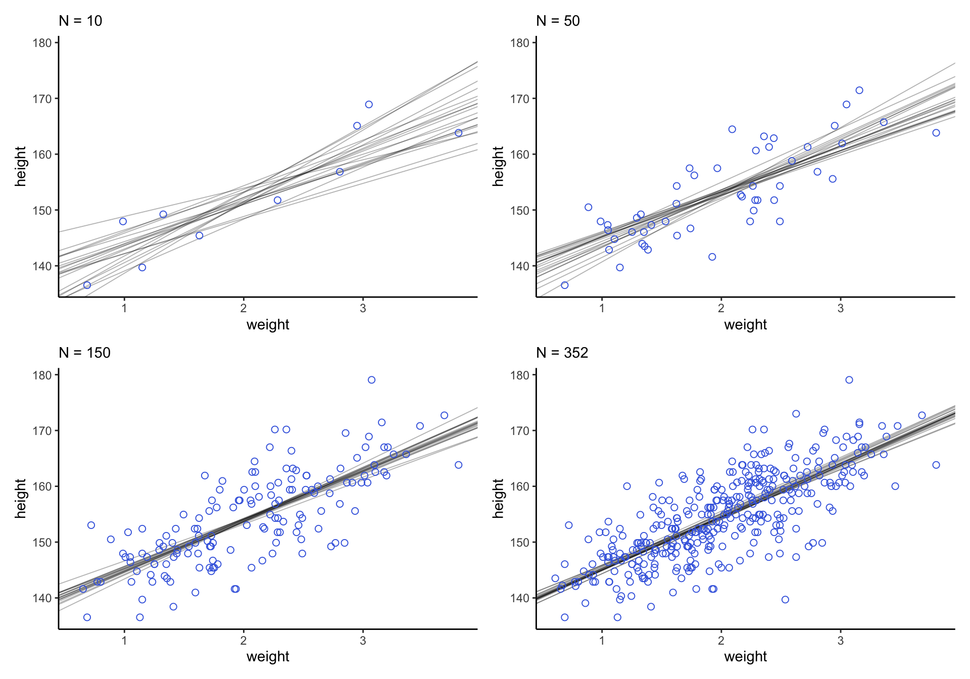
圖 46.20: Samples from the quadratic approximate posterior distribution for the height/weight model with 20 to 352 (increasing) samples of data. 20 Lines sampled from the posterior distribution.
可以看見,當數據越多,事後直線估計給出的穩定性越好,不確定性越小。
post <- extract.samples( m4.3 )
mu_at50 <- post$a + post$b * (50 - xbar)
head(mu_at50)
## [1] 159.31803 158.83253 159.06214 158.61510 159.37716 158.89217也就是說,當體重為 50 kg 時,身高的事後概率分佈可以繪製為:
dens(mu_at50, col = rangi2, lwd = 2, xlab = "mu | weight = 50")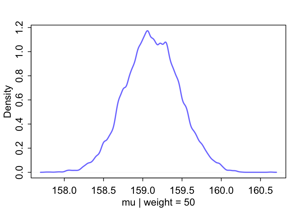
圖 46.21: The quadratic approximate posterior distribution of the mean height, when weight is 50 kg.
相似的,完成上述圖形的不同代碼可以寫作:
mu_at_50 <- postb %>%
  transmute(mu_at_50 = b_Intercept + b_weight_c + 5.01)

head(mu_at_50)
## mu_at_50
## 1 159.93786
## 2 160.89784
## 3 160.13896
## 4 160.37301
## 5 160.63488
## 6 160.35699mu_at_50 %>%
ggplot(aes(x = mu_at_50, y = 0)) +
stat_halfeye(point_interval = mode_hdi, .width = .95,
fill = "royalblue") +
scale_y_continuous(NULL, breaks = NULL) +
xlab(expression(mu["height | weight = 50"])) +
theme_classic()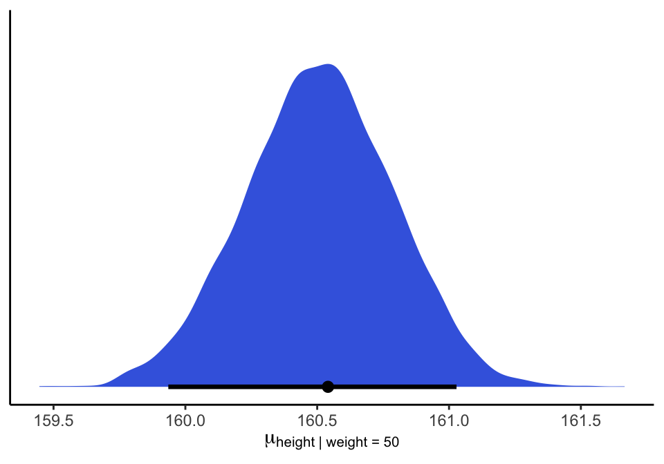
圖 46.22: The quadratic approximate posterior distribution of the mean height, when weight is 50 kg.
如果說你要給他增加一個可信區間,那麼當體重為 50 kg時,身高的事後預測89% 區間是:
PI(mu_at50, prob = 0.89)## 5% 94%
## 158.56552 159.68080但是其實我們更希望使用這事後概率分佈來繪製平均事後截距,平均事後斜率給出的直線本身的不確定性(也就是這條直線本身的89%區間)。函數 link() 提供了每一名參加實驗對象的事後身高均值的分佈。
mu <- link( m4.3 )
str(mu)
## num [1:1000, 1:352] 158 158 157 157 157 ...然後我們使用一段體重的區間來做身高的預測值:
# define sequence of weights to compute predictions for
# these values will be on the horizontal axis

weight.seq <- seq( from = 25, to = 70, by = 1)
使用 link() 函數來計算這些體重的事後身高分佈:
# use link to compute mu
# for each sample from posterior
# and for each weight in weight.seq

mu <- link(m4.3, data = data.frame(weight = weight.seq))
str(mu)
## num [1:1000, 1:46] 136 137 137 136 138 ...繪製這些體重值上的預測事後身高均值:
# use type = "n" to hide raw data
plot( height ~ weight, d2, type = "n")

# loop over samples and plot each mu value

for ( i in 1:100)
  points( weight.seq, mu[i, ], pch = 16, col = col.alpha(rangi2, 0.1))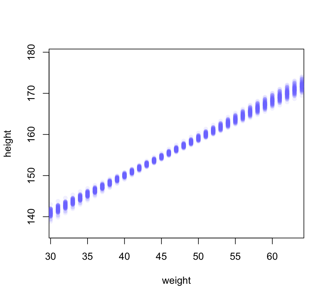
圖 46.23: The first 100 values in the distribution of mu at each weight value.
可以看到每一個體重點上的事後身高預測分佈都是一個類似圖 46.21 那樣的正(常)態分佈。而且也能注意到,身高的事後分佈的不確定性,他們每一個體重值上的事後身高分佈的方差其實是根據不同的身高而有大小區別之分。
# summarize the distribution of mu
mu.mean <- apply( mu, 2, mean )
mu.PI <- apply( mu, 2, PI, prob = 0.89)

# plot raw data
# fading out points to make line and interval more visible
plot( height ~ weight, data = d2, col = col.alpha(rangi2, 0.5))

# plot the MAP line, aka the mean mu for each weight
lines( weight.seq, mu.mean )

# plot a shaded region for 89% PI

shade( mu.PI, weight.seq )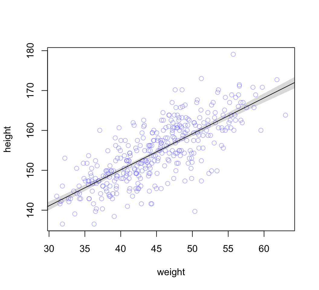
圖 46.24: The height data with 89% compatibility interval of the mean indicated by the shaded region. Compare this region to the distributions of blue points.
考慮身高本身的方差進來:
sim.height <- sim(m4.3, data = list(weight = weight.seq))
str(sim.height)
## num [1:1000, 1:46] 137 145 131 134 143 ...height.PI <- apply( sim.height, 2, PI, prob = 0.89)
# plot raw data
plot( height ~ weight, d2, col = col.alpha(rangi2, 0.5))
# draw MAP line
lines( weight.seq, mu.mean )
# draw HPDI region for line
# mu.HPDI <- HPDI()
shade( mu.PI, weight.seq )
# draw PI for simulated heights
shade( height.PI, weight.seq)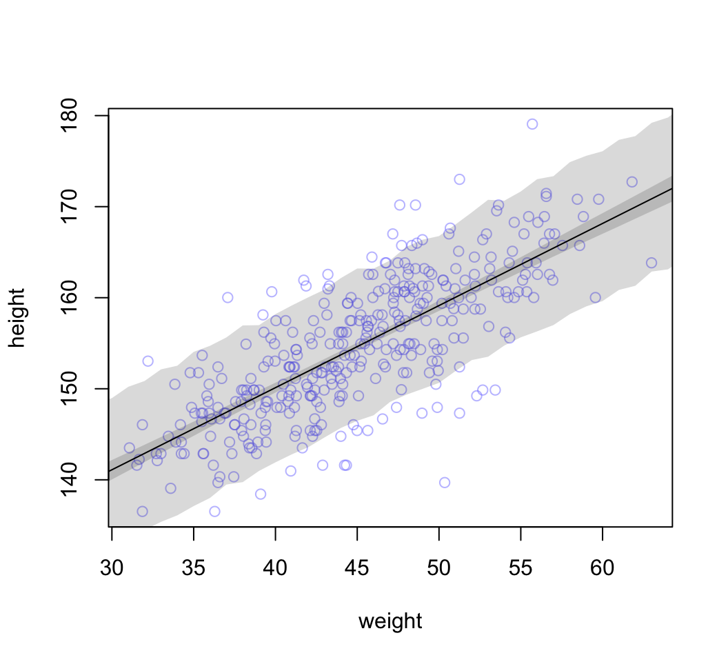
圖 46.25: 89% prediction interval for height, as a function of weight. The solid line is the average line for the mean height at each weight. The two shaded regions show different 89% plausible regions. The narrow shaded interval around the line is the distribution of mu. The wider shaded region represents the region within which the model expects to find 89% of actual heights in the population, at each weight.