Rstan Wonderful R-(4)
邏輯回歸模型的 Rstan 貝葉斯實現
本小節使用的數據,和前一節的出勤率數據很類似:
d <- read.table("https://raw.githubusercontent.com/winterwang/RStanBook/master/chap05/input/data-attendance-2.txt",
                     sep = ",", header = T)
head(d)
## PersonID A Score M Y
## 1 1 0 69 43 38
## 2 2 1 145 56 40
## 3 3 0 125 32 24
## 4 4 1 86 45 33
## 5 5 1 158 33 23
## 6 6 0 133 61 60其中,
PersonID: 是學生的編號;A,Score: 和之前一樣用來預測出勤率的兩個預測變量,分別是表示是否喜歡打工的A,和表示對學習本身是否喜歡的評分 (滿分200);M: 過去三個月內,該名學生一共需要上課的總課時數;Y: 過去三個月內,該名學生實際上出勤的課時數。
確定分析目的
需要回答的問題依然是,\(A, Score\) 分別在多大程度上預測學生的出勤率?另外,我們希望知道的是,當需要修的課時數固定的事後,這兩個預測變量能準確提供 \(Y\) 的多少信息?
確認數據分佈
library(ggplot2)
library(GGally)

set.seed(1)
d <- d[, -1]
# d <- read.csv(file='input/data-attendance-2.txt')[,-1]
d$A <- as.factor(d$A)
d <- transform(d, ratio=Y/M)
N_col <- ncol(d)
ggp <- ggpairs(d, upper='blank', diag='blank', lower='blank')

for(i in 1:N_col) {
  x <- d[,i]
  p <- ggplot(data.frame(x, A=d$A), aes(x))
  p <- p + theme_bw(base_size=14)
  p <- p + theme(axis.text.x=element_text(angle=40, vjust=1, hjust=1))
  if (class(x) == 'factor') {
    p <- p + geom_bar(aes(fill=A), color='grey20')
  } else {
    bw <- (max(x)-min(x))/10
    p <- p + geom_histogram(aes(fill=A), color='grey20', binwidth=bw)
    p <- p + geom_line(eval(bquote(aes(y=..count..*.(bw)))), stat='density')
  }
  p <- p + geom_label(data=data.frame(x=-Inf, y=Inf, label=colnames(d)[i]), aes(x=x, y=y, label=label), hjust=0, vjust=1)
  p <- p + scale_fill_manual(values=alpha(c('white', 'grey40'), 0.5))
  ggp <- putPlot(ggp, p, i, i)
}

zcolat <- seq(-1, 1, length=81)
zcolre <- c(zcolat[1:40]+1, rev(zcolat[41:81]))

for(i in 1:(N_col-1)) {
  for(j in (i+1):N_col) {
    x <- as.numeric(d[,i])
    y <- as.numeric(d[,j])
    r <- cor(x, y, method='spearman', use='pairwise.complete.obs')
    zcol <- lattice::level.colors(r, at=zcolat, col.regions=grey(zcolre))
    textcol <- ifelse(abs(r) < 0.4, 'grey20', 'white')
    ell <- ellipse::ellipse(r, level=0.95, type='l', npoints=50, scale=c(.2, .2), centre=c(.5, .5))
    p <- ggplot(data.frame(ell), aes(x=x, y=y))
    p <- p + theme_bw() + theme(
      plot.background=element_blank(),
      panel.grid.major=element_blank(), panel.grid.minor=element_blank(),
      panel.border=element_blank(), axis.ticks=element_blank()
    )
    p <- p + geom_polygon(fill=zcol, color=zcol)
    p <- p + geom_text(data=NULL, x=.5, y=.5, label=100*round(r, 2), size=6, col=textcol)
    ggp <- putPlot(ggp, p, i, j)
  }
}

for(j in 1:(N_col-1)) {
  for(i in (j+1):N_col) {
    x <- d[,j]
    y <- d[,i]
    p <- ggplot(data.frame(x, y, gr=d$A), aes(x=x, y=y, fill=gr, shape=gr))
    p <- p + theme_bw(base_size=14)
    p <- p + theme(axis.text.x=element_text(angle=40, vjust=1, hjust=1))
    if (class(x) == 'factor') {
      p <- p + geom_boxplot(aes(group=x), alpha=3/6, outlier.size=0, fill='white')
      p <- p + geom_point(position=position_jitter(w=0.4, h=0), size=2)
    } else {
      p <- p + geom_point(size=2)
    }
    p <- p + scale_shape_manual(values=c(21, 24))
    p <- p + scale_fill_manual(values=alpha(c('white', 'grey40'), 0.5))
    ggp <- putPlot(ggp, p, i, j)
  }
}

ggp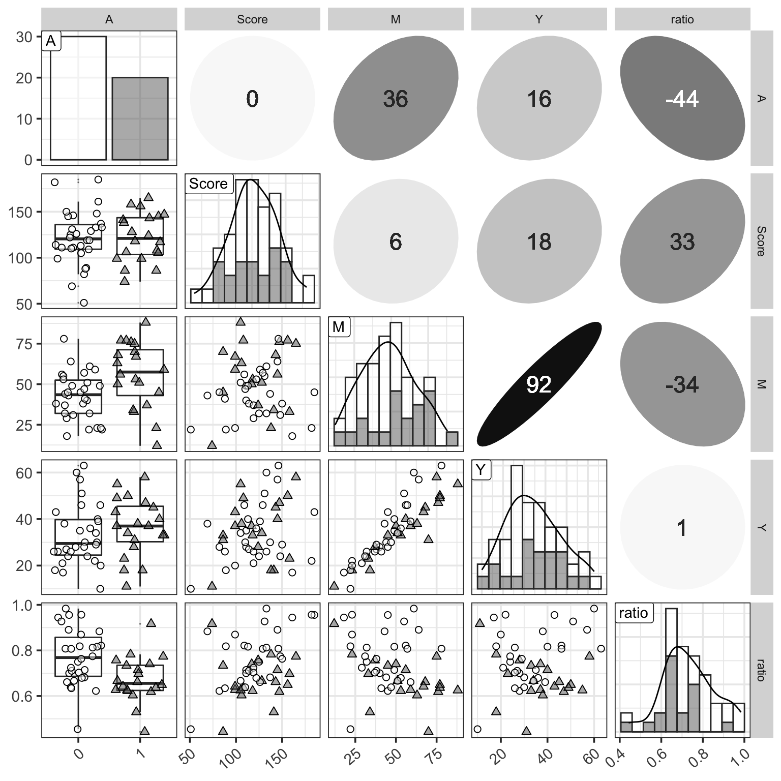
Figure 1: 三個變量的分佈觀察圖,相比之前增加了 \(ratio = Y/M\) 列。
從圖 1 還可以看出,由於總課時數越多,學生實際出勤的課時數也會越多所以 \(M, Y\) 兩者之間理應有很強的正相關。另外可能可以推測的是 \(Ratio\) 和是否愛學習的分數之間大概有可能有正相關,和是否喜歡打工之間大概可能有負相關。
寫下數學模型表達式
在 Stan 的語法中,使用的是反邏輯函數 (inverse logit): inv_logit 來描述下面的邏輯回歸模型 5-4。
\[ \begin{array}{l} q[n] = \text{inv_logit}(b_1 + b_2 A[n] + b_3Score[n]) & n = 1, 2, \dots, N \\ Y[n] \sim \text{Binomial}(M[n], q[n]) & n = 1, 2, \dots, N \\ \end{array} \]
上面的數學模型,可以被翻譯成下面的 Stan 語言:
data {
  int N;
  int<lower=0, upper=1> A[N];
  real<lower=0, upper=1> Score[N];
  int<lower=0> M[N];
  int<lower=0> Y[N];
}

parameters {
  real b1;
  real b2;
  real b3;
}

transformed parameters {
  real q[N];
  for (n in 1:N) {
    q[n] = inv_logit(b1 + b2*A[n] + b3*Score[n]);
  }
}

model {
  for (n in 1:N) {
    Y[n] ~ binomial(M[n], q[n]);
  }
}

generated quantities {
  real y_pred[N];
  for (n in 1:N) {
    y_pred[n] = binomial_rng(M[n], q[n]);
  }
}
下面的 R 代碼用來實現對上面 Stan 模型的擬合:
library(rstan)
d <- read.csv(file='https://raw.githubusercontent.com/winterwang/RStanBook/master/chap05/input/data-attendance-2.txt', header = T)
data <- list(N=nrow(d), A=d$A, Score=d$Score/200, M=d$M, Y=d$Y)
fit <- stan(file='stanfiles/model5-4.stan', data=data, seed=1234)
##
## SAMPLING FOR MODEL 'model5-4' NOW (CHAIN 1).
## Chain 1:
## Chain 1: Gradient evaluation took 1.9e-05 seconds
## Chain 1: 1000 transitions using 10 leapfrog steps per transition would take 0.19 seconds.
## Chain 1: Adjust your expectations accordingly!
## Chain 1:
## Chain 1:
## Chain 1: Iteration: 1 / 2000 [ 0%] (Warmup)
## Chain 1: Iteration: 200 / 2000 [ 10%] (Warmup)
## Chain 1: Iteration: 400 / 2000 [ 20%] (Warmup)
## Chain 1: Iteration: 600 / 2000 [ 30%] (Warmup)
## Chain 1: Iteration: 800 / 2000 [ 40%] (Warmup)
## Chain 1: Iteration: 1000 / 2000 [ 50%] (Warmup)
## Chain 1: Iteration: 1001 / 2000 [ 50%] (Sampling)
## Chain 1: Iteration: 1200 / 2000 [ 60%] (Sampling)
## Chain 1: Iteration: 1400 / 2000 [ 70%] (Sampling)
## Chain 1: Iteration: 1600 / 2000 [ 80%] (Sampling)
## Chain 1: Iteration: 1800 / 2000 [ 90%] (Sampling)
## Chain 1: Iteration: 2000 / 2000 [100%] (Sampling)
## Chain 1:
## Chain 1: Elapsed Time: 0.148218 seconds (Warm-up)
## Chain 1: 0.146931 seconds (Sampling)
## Chain 1: 0.295149 seconds (Total)
## Chain 1:
##
## SAMPLING FOR MODEL 'model5-4' NOW (CHAIN 2).
## Chain 2:
## Chain 2: Gradient evaluation took 1e-05 seconds
## Chain 2: 1000 transitions using 10 leapfrog steps per transition would take 0.1 seconds.
## Chain 2: Adjust your expectations accordingly!
## Chain 2:
## Chain 2:
## Chain 2: Iteration: 1 / 2000 [ 0%] (Warmup)
## Chain 2: Iteration: 200 / 2000 [ 10%] (Warmup)
## Chain 2: Iteration: 400 / 2000 [ 20%] (Warmup)
## Chain 2: Iteration: 600 / 2000 [ 30%] (Warmup)
## Chain 2: Iteration: 800 / 2000 [ 40%] (Warmup)
## Chain 2: Iteration: 1000 / 2000 [ 50%] (Warmup)
## Chain 2: Iteration: 1001 / 2000 [ 50%] (Sampling)
## Chain 2: Iteration: 1200 / 2000 [ 60%] (Sampling)
## Chain 2: Iteration: 1400 / 2000 [ 70%] (Sampling)
## Chain 2: Iteration: 1600 / 2000 [ 80%] (Sampling)
## Chain 2: Iteration: 1800 / 2000 [ 90%] (Sampling)
## Chain 2: Iteration: 2000 / 2000 [100%] (Sampling)
## Chain 2:
## Chain 2: Elapsed Time: 0.140054 seconds (Warm-up)
## Chain 2: 0.148312 seconds (Sampling)
## Chain 2: 0.288366 seconds (Total)
## Chain 2:
##
## SAMPLING FOR MODEL 'model5-4' NOW (CHAIN 3).
## Chain 3:
## Chain 3: Gradient evaluation took 9e-06 seconds
## Chain 3: 1000 transitions using 10 leapfrog steps per transition would take 0.09 seconds.
## Chain 3: Adjust your expectations accordingly!
## Chain 3:
## Chain 3:
## Chain 3: Iteration: 1 / 2000 [ 0%] (Warmup)
## Chain 3: Iteration: 200 / 2000 [ 10%] (Warmup)
## Chain 3: Iteration: 400 / 2000 [ 20%] (Warmup)
## Chain 3: Iteration: 600 / 2000 [ 30%] (Warmup)
## Chain 3: Iteration: 800 / 2000 [ 40%] (Warmup)
## Chain 3: Iteration: 1000 / 2000 [ 50%] (Warmup)
## Chain 3: Iteration: 1001 / 2000 [ 50%] (Sampling)
## Chain 3: Iteration: 1200 / 2000 [ 60%] (Sampling)
## Chain 3: Iteration: 1400 / 2000 [ 70%] (Sampling)
## Chain 3: Iteration: 1600 / 2000 [ 80%] (Sampling)
## Chain 3: Iteration: 1800 / 2000 [ 90%] (Sampling)
## Chain 3: Iteration: 2000 / 2000 [100%] (Sampling)
## Chain 3:
## Chain 3: Elapsed Time: 0.151245 seconds (Warm-up)
## Chain 3: 0.135369 seconds (Sampling)
## Chain 3: 0.286614 seconds (Total)
## Chain 3:
##
## SAMPLING FOR MODEL 'model5-4' NOW (CHAIN 4).
## Chain 4:
## Chain 4: Gradient evaluation took 8e-06 seconds
## Chain 4: 1000 transitions using 10 leapfrog steps per transition would take 0.08 seconds.
## Chain 4: Adjust your expectations accordingly!
## Chain 4:
## Chain 4:
## Chain 4: Iteration: 1 / 2000 [ 0%] (Warmup)
## Chain 4: Iteration: 200 / 2000 [ 10%] (Warmup)
## Chain 4: Iteration: 400 / 2000 [ 20%] (Warmup)
## Chain 4: Iteration: 600 / 2000 [ 30%] (Warmup)
## Chain 4: Iteration: 800 / 2000 [ 40%] (Warmup)
## Chain 4: Iteration: 1000 / 2000 [ 50%] (Warmup)
## Chain 4: Iteration: 1001 / 2000 [ 50%] (Sampling)
## Chain 4: Iteration: 1200 / 2000 [ 60%] (Sampling)
## Chain 4: Iteration: 1400 / 2000 [ 70%] (Sampling)
## Chain 4: Iteration: 1600 / 2000 [ 80%] (Sampling)
## Chain 4: Iteration: 1800 / 2000 [ 90%] (Sampling)
## Chain 4: Iteration: 2000 / 2000 [100%] (Sampling)
## Chain 4:
## Chain 4: Elapsed Time: 0.144055 seconds (Warm-up)
## Chain 4: 0.144297 seconds (Sampling)
## Chain 4: 0.288352 seconds (Total)
## Chain 4:fit## Inference for Stan model: model5-4.
## 4 chains, each with iter=2000; warmup=1000; thin=1;
## post-warmup draws per chain=1000, total post-warmup draws=4000.
##
## mean se_mean sd 2.5% 25% 50% 75% 97.5%
## b1 0.09 0.01 0.23 -0.33 -0.08 0.08 0.25 0.53
## b2 -0.62 0.00 0.10 -0.82 -0.69 -0.62 -0.56 -0.44
## b3 1.91 0.01 0.37 1.19 1.66 1.91 2.17 2.61
## q[1] 0.68 0.00 0.02 0.63 0.66 0.68 0.70 0.73
## q[2] 0.70 0.00 0.02 0.67 0.69 0.70 0.71 0.73
## q[3] 0.78 0.00 0.01 0.76 0.77 0.78 0.79 0.81
## q[4] 0.57 0.00 0.02 0.53 0.56 0.57 0.59 0.61
## q[5] 0.73 0.00 0.02 0.69 0.71 0.73 0.74 0.76
## q[6] 0.80 0.00 0.01 0.77 0.79 0.80 0.80 0.82
## q[7] 0.76 0.00 0.01 0.73 0.75 0.76 0.77 0.78
## q[8] 0.70 0.00 0.02 0.67 0.69 0.70 0.72 0.74
## q[9] 0.81 0.00 0.01 0.79 0.81 0.82 0.82 0.84
## q[10] 0.81 0.00 0.01 0.79 0.80 0.81 0.82 0.84
## q[11] 0.69 0.00 0.02 0.66 0.68 0.69 0.70 0.72
## q[12] 0.80 0.00 0.01 0.78 0.79 0.80 0.81 0.83
## q[13] 0.64 0.00 0.02 0.61 0.63 0.64 0.65 0.67
## q[14] 0.76 0.00 0.01 0.73 0.75 0.76 0.77 0.78
## q[15] 0.76 0.00 0.01 0.73 0.75 0.76 0.76 0.78
## q[16] 0.60 0.00 0.02 0.56 0.59 0.60 0.61 0.64
## q[17] 0.76 0.00 0.01 0.74 0.76 0.76 0.77 0.79
## q[18] 0.70 0.00 0.02 0.67 0.69 0.70 0.72 0.74
## q[19] 0.86 0.00 0.02 0.83 0.85 0.86 0.88 0.89
## q[20] 0.72 0.00 0.02 0.69 0.71 0.72 0.73 0.76
## q[21] 0.57 0.00 0.02 0.53 0.56 0.57 0.59 0.61
## q[22] 0.62 0.00 0.02 0.59 0.61 0.62 0.63 0.65
## q[23] 0.62 0.00 0.02 0.58 0.61 0.62 0.63 0.65
## q[24] 0.70 0.00 0.02 0.67 0.69 0.70 0.71 0.73
## q[25] 0.64 0.00 0.02 0.61 0.63 0.64 0.65 0.67
## q[26] 0.67 0.00 0.01 0.64 0.66 0.67 0.68 0.69
## q[27] 0.77 0.00 0.01 0.75 0.76 0.77 0.78 0.80
## q[28] 0.77 0.00 0.01 0.75 0.76 0.77 0.78 0.80
## q[29] 0.84 0.00 0.01 0.81 0.83 0.84 0.85 0.86
## q[30] 0.76 0.00 0.01 0.74 0.75 0.76 0.77 0.79
## q[31] 0.74 0.00 0.02 0.70 0.73 0.74 0.75 0.78
## q[32] 0.54 0.00 0.03 0.49 0.52 0.54 0.56 0.60
## q[33] 0.69 0.00 0.02 0.66 0.68 0.69 0.70 0.72
## q[34] 0.66 0.00 0.01 0.63 0.65 0.66 0.67 0.69
## q[35] 0.78 0.00 0.01 0.76 0.78 0.78 0.79 0.81
## q[36] 0.79 0.00 0.01 0.77 0.78 0.79 0.80 0.82
## q[37] 0.62 0.00 0.02 0.58 0.60 0.62 0.63 0.65
## q[38] 0.76 0.00 0.01 0.73 0.75 0.76 0.77 0.78
## q[39] 0.72 0.00 0.02 0.69 0.71 0.72 0.73 0.75
## q[40] 0.72 0.00 0.02 0.68 0.70 0.72 0.73 0.75
## q[41] 0.79 0.00 0.01 0.77 0.78 0.79 0.80 0.81
## q[42] 0.80 0.00 0.01 0.77 0.79 0.80 0.80 0.82
## q[43] 0.78 0.00 0.01 0.75 0.77 0.78 0.79 0.80
## q[44] 0.82 0.00 0.01 0.79 0.81 0.82 0.83 0.84
## q[45] 0.86 0.00 0.02 0.83 0.85 0.86 0.87 0.89
## q[46] 0.75 0.00 0.01 0.72 0.74 0.75 0.76 0.78
## q[47] 0.64 0.00 0.03 0.58 0.62 0.64 0.66 0.70
## q[48] 0.82 0.00 0.01 0.79 0.81 0.82 0.83 0.85
## q[49] 0.74 0.00 0.02 0.71 0.73 0.74 0.75 0.77
## q[50] 0.60 0.00 0.02 0.56 0.59 0.60 0.61 0.64
## y_pred[1] 29.07 0.06 3.26 23.00 27.00 29.00 31.00 35.00
## y_pred[2] 39.29 0.06 3.57 32.00 37.00 39.00 42.00 46.00
## y_pred[3] 25.03 0.04 2.38 20.00 23.00 25.00 27.00 29.00
## y_pred[4] 25.78 0.06 3.48 19.00 23.00 26.00 28.00 32.00
## y_pred[5] 23.85 0.04 2.62 19.00 22.00 24.00 26.00 29.00
## y_pred[6] 48.57 0.05 3.17 42.00 47.00 49.00 51.00 54.00
## y_pred[7] 37.24 0.05 3.03 31.00 35.00 37.00 39.00 43.00
## y_pred[8] 53.52 0.07 4.13 45.00 51.00 54.00 56.00 61.00
## y_pred[9] 63.60 0.06 3.57 56.00 61.00 64.00 66.00 70.00
## y_pred[10] 52.03 0.05 3.21 46.00 50.00 52.00 54.00 58.00
## y_pred[11] 23.56 0.05 2.73 18.00 22.00 24.00 25.00 29.00
## y_pred[12] 35.20 0.04 2.67 30.00 33.00 35.00 37.00 40.00
## y_pred[13] 34.12 0.06 3.61 27.00 32.00 34.00 37.00 41.00
## y_pred[14] 30.40 0.04 2.79 25.00 29.00 30.50 32.00 36.00
## y_pred[15] 42.26 0.05 3.28 36.00 40.00 42.00 45.00 48.00
## y_pred[16] 35.48 0.06 3.84 28.00 33.00 36.00 38.00 43.00
## y_pred[17] 29.07 0.04 2.72 23.00 27.00 29.00 31.00 34.00
## y_pred[18] 31.72 0.05 3.20 25.00 30.00 32.00 34.00 38.00
## y_pred[19] 38.83 0.04 2.41 34.00 37.00 39.00 41.00 43.00
## y_pred[20] 55.53 0.07 4.16 47.00 53.00 56.00 58.00 63.00
## y_pred[21] 40.00 0.07 4.41 31.00 37.00 40.00 43.00 49.00
## y_pred[22] 47.90 0.07 4.38 39.00 45.00 48.00 51.00 56.00
## y_pred[23] 38.95 0.06 4.00 31.00 36.00 39.00 42.00 46.00
## y_pred[24] 47.35 0.06 3.91 39.00 45.00 47.00 50.00 55.00
## y_pred[25] 32.06 0.05 3.41 25.00 30.00 32.00 34.00 39.00
## y_pred[26] 34.00 0.06 3.48 27.00 32.00 34.00 36.00 41.00
## y_pred[27] 22.38 0.04 2.33 17.00 21.00 22.00 24.00 27.00
## y_pred[28] 28.58 0.04 2.66 23.00 27.00 29.00 30.00 34.00
## y_pred[29] 15.06 0.03 1.56 12.00 14.00 15.00 16.00 18.00
## y_pred[30] 37.36 0.05 3.04 31.00 35.00 37.00 39.00 43.00
## y_pred[31] 55.39 0.07 4.07 47.00 53.00 56.00 58.00 63.00
## y_pred[32] 6.48 0.03 1.72 3.00 5.00 6.00 8.00 10.00
## y_pred[33] 15.74 0.03 2.23 11.00 14.00 16.00 17.00 20.00
## y_pred[34] 24.36 0.05 2.90 18.98 22.00 24.00 26.00 30.00
## y_pred[35] 46.30 0.05 3.26 40.00 44.00 46.00 49.00 52.00
## y_pred[36] 43.46 0.05 3.05 37.00 41.00 44.00 46.00 49.00
## y_pred[37] 54.13 0.08 4.80 45.00 51.00 54.00 57.00 63.00
## y_pred[38] 35.67 0.05 3.05 29.00 34.00 36.00 38.00 41.00
## y_pred[39] 15.85 0.04 2.13 11.00 14.00 16.00 17.00 20.00
## y_pred[40] 29.35 0.05 2.99 23.00 27.00 29.00 31.00 35.00
## y_pred[41] 45.02 0.05 3.19 39.00 43.00 45.00 47.00 51.00
## y_pred[42] 25.48 0.04 2.30 21.00 24.00 26.00 27.00 30.00
## y_pred[43] 41.32 0.05 3.11 35.00 39.00 41.00 43.00 47.00
## y_pred[44] 25.32 0.04 2.25 21.00 24.00 25.00 27.00 29.00
## y_pred[45] 19.79 0.03 1.74 16.00 19.00 20.00 21.00 23.00
## y_pred[46] 38.19 0.05 3.23 31.00 36.00 38.00 40.00 44.00
## y_pred[47] 14.04 0.04 2.40 9.00 12.00 14.00 16.00 19.00
## y_pred[48] 31.19 0.04 2.42 26.00 30.00 31.00 33.00 36.00
## y_pred[49] 16.95 0.03 2.12 12.00 16.00 17.00 18.00 21.00
## y_pred[50] 40.32 0.07 4.27 32.00 37.00 40.00 43.00 48.03
## lp__ -1389.42 0.04 1.21 -1392.48 -1390.00 -1389.12 -1388.51 -1387.97
## n_eff Rhat
## b1 1238 1.01
## b2 1892 1.00
## b3 1161 1.01
## q[1] 1504 1.01
## q[2] 2126 1.00
## q[3] 2604 1.00
## q[4] 1454 1.00
## q[5] 1799 1.00
## q[6] 2443 1.00
## q[7] 2449 1.00
## q[8] 2065 1.00
## q[9] 1992 1.00
## q[10] 2036 1.00
## q[11] 2258 1.00
## q[12] 2332 1.00
## q[13] 2512 1.00
## q[14] 2449 1.00
## q[15] 2389 1.00
## q[16] 1727 1.00
## q[17] 2528 1.00
## q[18] 1667 1.00
## q[19] 1350 1.01
## q[20] 1839 1.00
## q[21] 1454 1.00
## q[22] 2083 1.00
## q[23] 1989 1.00
## q[24] 2191 1.00
## q[25] 2480 1.00
## q[26] 2618 1.00
## q[27] 2611 1.00
## q[28] 2611 1.00
## q[29] 1588 1.00
## q[30] 2504 1.00
## q[31] 1684 1.00
## q[32] 1329 1.01
## q[33] 2360 1.00
## q[34] 2628 1.00
## q[35] 2591 1.00
## q[36] 2494 1.00
## q[37] 1945 1.00
## q[38] 2419 1.00
## q[39] 1808 1.00
## q[40] 1785 1.00
## q[41] 2539 1.00
## q[42] 2443 1.00
## q[43] 2622 1.00
## q[44] 1910 1.00
## q[45] 1369 1.00
## q[46] 2260 1.00
## q[47] 1389 1.01
## q[48] 1840 1.00
## q[49] 2073 1.00
## q[50] 1727 1.00
## y_pred[1] 3373 1.00
## y_pred[2] 3405 1.00
## y_pred[3] 4073 1.00
## y_pred[4] 3876 1.00
## y_pred[5] 3753 1.00
## y_pred[6] 4028 1.00
## y_pred[7] 3672 1.00
## y_pred[8] 3782 1.00
## y_pred[9] 3937 1.00
## y_pred[10] 3629 1.00
## y_pred[11] 3662 1.00
## y_pred[12] 3836 1.00
## y_pred[13] 3918 1.00
## y_pred[14] 3986 1.00
## y_pred[15] 3819 1.00
## y_pred[16] 3824 1.00
## y_pred[17] 4008 1.00
## y_pred[18] 3713 1.00
## y_pred[19] 3338 1.00
## y_pred[20] 3292 1.00
## y_pred[21] 3463 1.00
## y_pred[22] 3943 1.00
## y_pred[23] 3884 1.00
## y_pred[24] 3653 1.00
## y_pred[25] 4050 1.00
## y_pred[26] 3863 1.00
## y_pred[27] 3952 1.00
## y_pred[28] 3686 1.00
## y_pred[29] 3824 1.00
## y_pred[30] 3953 1.00
## y_pred[31] 3577 1.00
## y_pred[32] 3957 1.00
## y_pred[33] 4101 1.00
## y_pred[34] 3888 1.00
## y_pred[35] 3968 1.00
## y_pred[36] 3967 1.00
## y_pred[37] 3709 1.00
## y_pred[38] 3809 1.00
## y_pred[39] 3665 1.00
## y_pred[40] 3418 1.00
## y_pred[41] 3991 1.00
## y_pred[42] 4050 1.00
## y_pred[43] 4147 1.00
## y_pred[44] 3604 1.00
## y_pred[45] 3786 1.00
## y_pred[46] 3640 1.00
## y_pred[47] 2938 1.00
## y_pred[48] 3762 1.00
## y_pred[49] 4067 1.00
## y_pred[50] 3501 1.00
## lp__ 1107 1.00
##
## Samples were drawn using NUTS(diag_e) at Mon May 18 16:53:57 2020.
## For each parameter, n_eff is a crude measure of effective sample size,
## and Rhat is the potential scale reduction factor on split chains (at
## convergence, Rhat=1).把獲得的參數事後樣本的均值代入上面的數學模型中可得:
\[ \begin{array}{l} q[n] = \text{inv_logit}(0.09 - 0.62 A[n] + 1.90Score[n]) & n = 1, 2, \dots, N \\ Y[n] \sim \text{Binomial}(M[n], q[n]) & n = 1, 2, \dots, N \\ \end{array} \]
確認收斂效果
library(bayesplot)

color_scheme_set("mix-brightblue-gray")

posterior2 <- rstan::extract(fit, inc_warmup = TRUE, permuted = FALSE)

p <- mcmc_trace(posterior2, n_warmup = 0, pars = c("b1", "b2", "b3", "lp__"),
                facet_args = list(nrow = 2, labeller = label_parsed))
p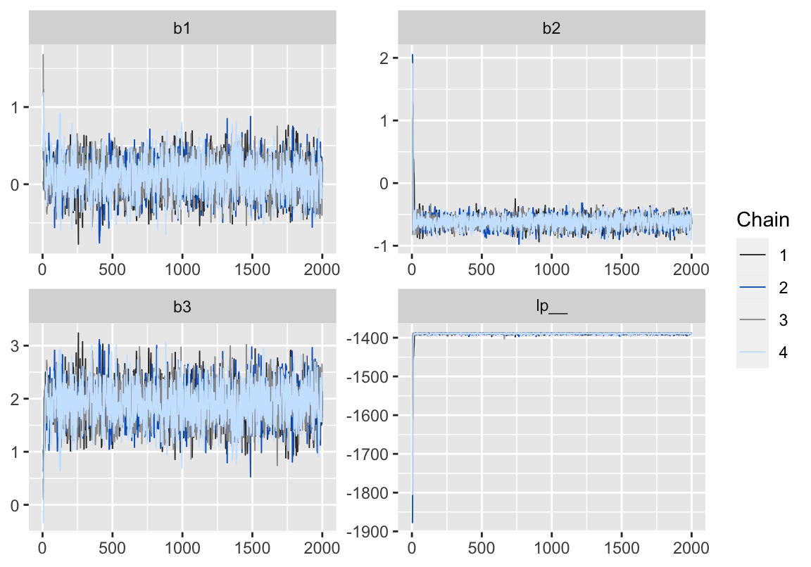
Figure 2: 用 bayesplot包數繪製的模型5-3的MCMC鏈式軌跡圖 (trace plot)。
ms <- rstan::extract(fit)

d_qua <- t(apply(ms$y_pred, 2, quantile, prob=c(0.1, 0.5, 0.9)))
colnames(d_qua) <- c('p10', 'p50', 'p90')
d_qua <- data.frame(d, d_qua)
d_qua$A <- as.factor(d_qua$A)

p <- ggplot(data=d_qua, aes(x=Y, y=p50, ymin=p10, ymax=p90, shape=A, fill=A))
p <- p + theme_bw(base_size=18) + theme(legend.key.height=grid::unit(2.5,'line'))
p <- p + coord_fixed(ratio=1, xlim=c(5, 70), ylim=c(5, 70))
p <- p + geom_pointrange(size=0.8, color='grey5')
p <- p + geom_abline(aes(slope=1, intercept=0), color='black', alpha=3/5, linetype='31')
p <- p + scale_shape_manual(values=c(21, 24))
p <- p + scale_fill_manual(values=c('white', 'grey70'))
p <- p + labs(x='Observed', y='Predicted')
p <- p + scale_x_continuous(breaks=seq(from=0, to=70, by=20))
p <- p + scale_y_continuous(breaks=seq(from=0, to=70, by=20))
p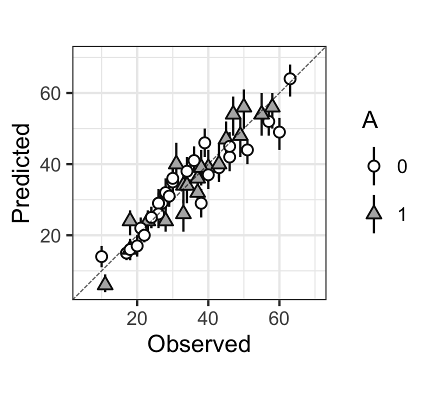
Figure 3: 觀測值(x),和預測值(y)的散點圖,以及預測值的80%預測區間。